Dynamic Plots Using an Equation Function
Anonym
This blog post continues to explore the Dynamic Visualizations available using the Equation argument on the PLOT function. In this example, we explore the use of a function name rather than an equation string. See Dynamic Plots Using an Equation String for the first article in this series.
Using an equation string has some limitations:
- You can only have a single statement
- You cannot easily change the equation unless you set a new string
- You cannot pass parameters into your equation
As a different approach, create an IDL function containing your equation and then pass the function name to the Equation argument. This method allows you a bit more flexibility in your input equations.
For example, in the first line of the code above, we could have simply written:
p1= PLOT('LambertW', '2', DIMENSIONS=[400,400],$
NAME='Upperbranch', $
TITLE='LambertW Function', XRANGE=[-0.4, 2])
Notice that we no longer have an X variable in our equation, we just have the name of the function. We can also create our own routine which accepts our X vector and some optional user data.
First, create a new IDL routine called ex_plot_function and save it in a file ex_plot_function.pro on IDL's path:
FUNCTIONex_plot_function, x, k
COMPILE_OPTIDL2
RETURN,LAMBERTW(DCOMPLEX(x), k)
END
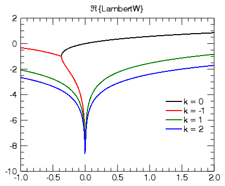
Next, we create our plot visualization, passing in the name of our equation along with our user data containing the "branch" parameter k:
p1= PLOT('ex_plot_function', '2', DIMENSIONS=[400,400],$
NAME='k= 0', EQN_USERDATA=0, $
TITLE='$\Re${LambertW}',XRANGE=[-1, 2])
p2r= PLOT('ex_plot_function', '2r', /OVERPLOT, $
NAME='k= -1', EQN_USERDATA=-1)
p3r= PLOT('ex_plot_function', '2g', /OVERPLOT, $
NAME='k= 1', EQN_USERDATA=1)
p4r= PLOT('ex_plot_function', '2b', /OVERPLOT, $
NAME='k= 2', EQN_USERDATA=2)
lg= LEGEND(/DATA, POSITION=[1.9, -4], LINESTYLE=6, SHADOW=0)
Our plot should now look like the following:

Again, we can pan and zoom around the plot, and IDL will automatically update the equations.