The Spectral Hourglass Workflow Series

Part 1, An Introduction

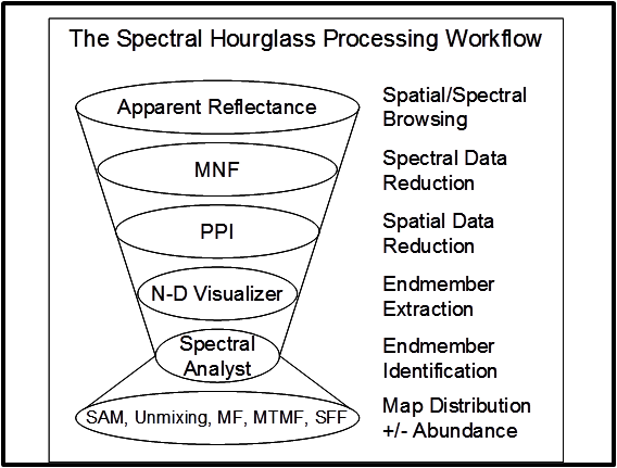
For the next several months, I will be publishing blog posts regarding the Spectral Hourglass Workflow, employed in many hyperspectral analysis workflows. This will be informally referred to as the Spectral Hourglass Workflow Series (SHWS). The figure below depicts the general order one would follow when analyzing a hyperspectral dataset. There will be a minimum of one blog post per ‘part’; Spatial/Spectral Browsing (1), Spectral Data Reduction (2), Spatial Data Reduction (3), Endmember Extraction (4), Endmember Identification (5) and finally Mapping Distribution and/or Abundance (6).

This blog series is mainly intended for beginner-intermediate level users. Although advanced users will find this helpful, especially as it pertains to the functionality available within ENVI, we will not be getting into the weeds about the research surrounding the various algorithms. Each part of this SHWS focuses on how each step of the workflow can be accomplished within ENVI, along with background information regarding that step and the algorithms utilized.

So who would typically utilize this Spectral Hourglass Workflow and why? The short answer to this question would be anyone working with Hyperspectral Imagery (HSI) wishing to map the distribution or abundance of specific materials within a scene. A great example of this would be a geologist attempting to identify the presence of certain minerals for excavation/mining purposes.

The overall goal of this workflow is to identify endmembers, also known as materials that are spectrally unique in the wavelength bands used to collect the image. In essence an endmember is a pixel representing one specific type of material; say a specific type of mineral.

The vast majority of pixels in any scene will contain mixed spectra from various materials surrounding that exact location (pixel) on the surface of the earth. If one can identify pure pixels in the scene, be it for vegetation, geology, identification, or a litany of other uses, then one can also map the abundance of those pixels within the scene. Geologists want to identify regions on the surface of the earth where the composition of minerals are very pure, as the more pure a mineral is the less sorting and extraction work needed to be able to eventually sell said mineral. Being able to extract the most pure spectra will also allow a user to build spectral libraries built from in-scene data, which is a great resource for material detection and identification in areas with features.

This is but a brief introduction to the Spectral Hourglass Workflow and the world of hyperspectral data analysis. HSI sensors are not only becoming more widely used, but the cost of the data they collect is beginning to reduce drastically when compared to even five years prior. ENVI boasts the best in class HSI analysis capabilities, and this several-part series will detail exactly why this is the case, as well as help you get up to speed on the proper tactics to best extract useful information from hyperspectral datasets.

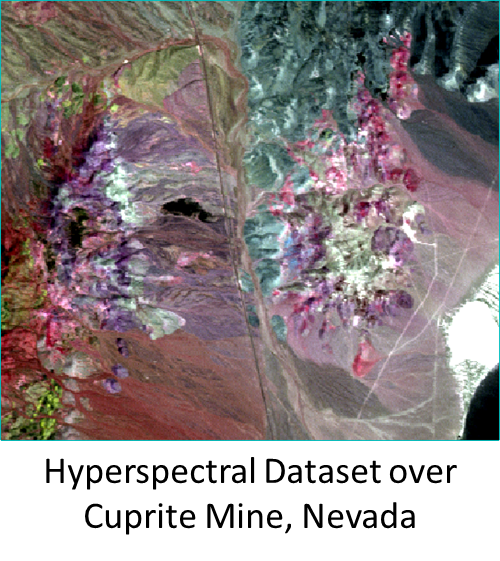
An added bonus of this series is that we will be stepping through each part of this workflow with the same dataset, and this data is shipped with every instance of ENVI. The specific file location on your disk will vary depending on how you installed ENVI, but the Cuprite dataset we will be using throughout this blog series can be found in C:\ProgramFiles\Exelis\ENVI52\classic\data. The file name is ‘cup95eff.int’ and there is an associated header file found within the same folder. I look forward to taking you through the Spectral Hourglass Workflow step-by-step over the course of the next several months, please feel free to leave comments and questions regarding hyperspectral analysis!

Read The Spectral Hourglass Series: Part 2, Spatial/Spectral Browsing and Endmembers