Developing Custom Processing Algorithms with ENVI + IDL - It's So Easy!

 

Next week I will be teaching a class here in our Boulder, Colorado, office called Extending ENVI with IDL. Many people may not be aware that our geospatial image analysis software, ENVI, is built on a powerful programming language called IDL. IDL is used across disciplines to extract meaningful information and to create visualizations from complex numerical data. Predecessor versions of IDL were written for analysis of data from NASA missions such as Mariner and the International Ultraviolet Explorer. These predecessor versions of IDL were developed in the1970s at the Laboratory for Atmospheric and Space Physics (LASP) at the University of Colorado, Boulder. The first official version of IDL was released in 1977, by Research Systems Inc. (RSI). IDL has come a long way since it was first created in the 1970s. Our engineers are constantly adding new functionality to IDL to keep it modern, flexible, and user-friendly.

Because IDL has its roots as a programming language geared towards scientists and engineers working with multidimensional arrays of scientific data, it lends itself very naturally to working with raster data from remote sensing systems. In 1994, RSI released the first version of ENVI. Since then, ENVI and IDL have been like inseparable best friends. Whatever IDL can do, ENVI can too. ENVI has an API written in IDL that can be used to create custom algorithms, custom workflows, and for batch processing of remotely sensed data.

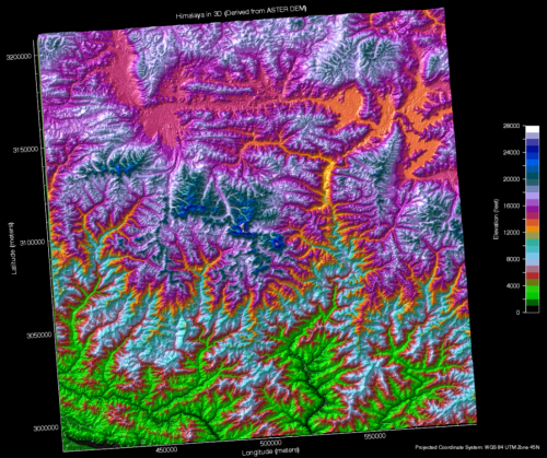
The ability of ENVI to be extended using IDL is, in my opinion, the single most powerful aspect of ENVI. The ENVI API has a quick learning curve and once you figure it out, the sky is the limit to what you can do with your data. This includes powerful visualizations of geographic data, such as the one I created below using the CONTOUR function.

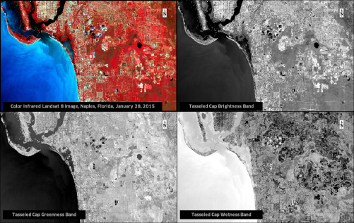
One of the more powerful aspects of the ENVI API is the ability to implement custom algorithms.This allows users to apply an algorithm that they have read about in scientific literature or to experiment with their own image analysis algorithms. Let’s go ahead and take a look at how one might implement a custom algorithm in ENVI using IDL. In this example, we will use the Tasseled Cap Transformation (TCT) for Landsat 8. The TCT was originally designed for the Landsat Multi-Spectral Scanner (MSS), which was launched in 1972. Subsequent adaptations of the TCT have been published in scientific literature for the Landsat Thematic Mapper (TM), the Landsat Enhanced Thematic Mapper (ETM) and the Landsat Enhanced Thematic Mapper Plus (ETM+) sensors. The ability to perform the TCT on Landsat MSS, TM, ETM and ETM+ images is available out-of-the-box with ENVI. However,the TCT algorithm for the Landsat Operational Land Imager (OLI) sensor was only recently published and has not yet made it into the ENVI Toolbox. But, because the algorithm is now available in the scientific literature, we can apply this algorithm to Landsat 8 data by using the ENVI API. This algorithm takes a Landsat 8 image and calculates a new image file containing 6 bands, with each band containing unique information about a scene, such as albedo (brightness), vegetation health (greenness), and water content (wetness).

The example code below can be implemented in ENVI + IDL to perform a TCT on Landsat 8 data, as described in an article titled, Derivations of a tasseled cap transformation based on Landsat 8 at-satellite reflectance:

; Copyright (c) 1988-2015, Exelis Visual Information Solutions, Inc. All rights reserved.

pro tasseledcapidl

 

; Set compile options - this is a standard compatibility line that is recommended for use in all IDL code

compile_opt IDL2

 

; Use the current session of ENVI

e=envi(/current)

 

; Path and filename to a pre-calibrated Landsat 8 image file

; Input file should be radiometrically calibrated and optionally atmospherically corrected

inputRaster = e.OpenRaster('C:\Data\Naples\LC80160422015028LGN00_RadCal_MS_Subset.dat')

 

; Subset the input raster - only these 6 bands are needed for the TCT calculation

subsetRaster=ENVIsubsetRaster(inputRaster, BANDS=[1,2,3,4,5,6])

 

; Set up output raster file

outputRaster = ENVIRaster(URI=outputURI, INHERITS_FROM=subsetRaster)

 

; Create tiles - creating tiles allows ENVI + IDL to iterate through the tiles, which is a good idea

; when you want to minimize the impact of image processing on your computer's resources

tiles = subsetRaster.CreateTileIterator(MODE='spectral')

 

; Iterate through tiles 

FOREACH tile, tiles DO BEGIN

; band 1 

b1 = tile[*,0]

; band 2

b2 = tile[*,1]

; band 3

b3 = tile[*,2]

; band 4

b4 = tile[*,3]

; band 5

b5 = tile[*,4]

; band 6

b6 = tile[*,5]

dims= size(tile,/DIMENSIONS)

data = make_array(dims,/FLOAT)

 

; Use IDL to do the TCT calculations

; Calculate brightness

data[*,0] = (b1 * 0.3029) + (b2 * 0.2786)+ (b3*0.4733) + (b4*0.5599) + (b5*0.508) + (b6*0.1872)

; Calculate greenness

data[*,1] = (b1 * (-0.2941)) + (b2 * (-0.243))+ (b3 * (-0.5424)) + (b4 * 0.7276) + (b5 * 0.0713)

; Calculate wetness

data[*,2] = (b1 * 0.1511) + (b2 * 0.1973)+ (b3 * 0.3283) + (b4 * 0.3407) + (b5 * (-0.7117)) + (b6*(-0.4559))

; Calculate TCT4 (Haze)

data[*,3] = (b1 * (-0.8239)) + (b2 * 0.0849)+ (b3 * 0.4396) + (b4 * (-0.058)) + (b5 * 0.2013) + (b6*(-0.2773))

; Calculate TCT5

data[*,4] = (b1 * (-0.3294)) + (b2 * 0.0557)+ (b3 * 0.1056) + (b4 * 0.1855) + (b5 * (-0.4349)) + (b6 *0.8085)

; Calculate TCT6

data[*,5] = (b1 * 0.1079) + (b2 * (-0.9023))+ (b3 * 0.4119) + (b4 * 0.0575) + (b5 * (-0.0259)) + (b6 *0.0252)

 

; Write to ouput file

outputRaster.SetTile, data, tiles

 

ENDFOREACH

 

; Add appropriate Band Names to the HDR file

metadata = outputRaster.METADATA

metadata.UpdateItem, 'BAND NAMES', ['Brightness','Greenness','Wetness','TCT4','TCT5','TCT6']

 

; Save changes to output file

outputRaster.save

 

; Display output file in ENVI Display

view=e.getview()

layer=view.createlayer(outputRaster)

 

end

 

The input file for this example was captured by Landsat 8 over Naples, Florida, on January 28, 2015. The screen capture below from the ENVI display shows a Color Infrared representation of the scene, along with the computed Brightness, Greenness and Wetness bands from the Tasseled Cap Transformation. This is just one example of how the power of IDL can make implementing custom algorithms so easy.

References:

Muhammad Hasan Ali Baig, Lifu Zhang, Tong Shuai & Qingxi Tong (2014) Derivations of a tasseled cap transformation based on Landsat 8 at-satellite reflectance, Remote Sensing Letters, 5:5, 423-431, DOI: 10.1080/2150704X.2014.915434