Lava, Plumes, and Machine Learning, Oh My!

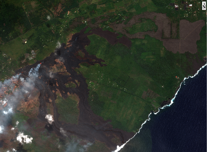
Recently, I downloaded a DigitalGlobe WorldView2 scene from GBDX and it just so happened that is was over Hawaii where Kilauea was recently erupting. In addition to this, the eruption was active when the scene was captured (May 23, 2018), so I was in for a surprise when I finally opened the image up and was able to see how powerful and destructive the eruption was. A subset of the scene situated directly over the eruption looked like this:

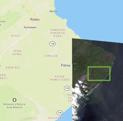
And for reference, here is a screenshot of the location of the image on a map with an overview of the original scene:

When I first looked at the scene, apart from the destruction, I had no idea that it would lead me down a path of creating some interesting analytics and classifiers in ENVI. Originally, I was just inspecting the RGB bands of the image and, when I switched to CIR to take a closer look at some of the vegetation next to the recent lava flows, I noticed that some of the lava was starting to glow:

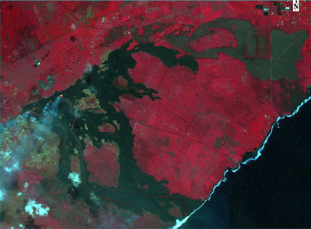
When I saw this, I decided I would look at a color composite of just the longer wavelengths and see what else would pop out. Because I was using WV2 data, I had 8 bands to choose from with two in the NIR range and one red edge band. When I inspected the RGB combination of NIR2 (950 nm), NIR1 (833 nm), and (725 nm) the lava really popped out!

After I saw this image, it got me thinking, could I extract the location of the molten lava, the cool lava, and the plume of gasses that were being emitted? I decided to take a look at doing this using state-of-the-art machine learning algorithms. If you are unfamiliar with the workflow for creating machine learning classifiers, it looks something like this:

1. Extract training data
2. Generate a classifier
3. Apply the classifier to the image and optionally iterate over training data based on performance

 

Now, if you have created a classifier before, you might know that the first and third step can take a very long time depending on the feature and algorithm being used. While that can be true, the machine learning algorithm that I decided to go with is a pixel based algorithm. Why does this matter? It means that we can very quickly, on the order of minutes, extract training data and generate a classifier for our data. In addition to this, some pixel based machine learning algorithms are very robust and perform well for satellite, aerial, and UAV data collection platforms even with large variations in classes (such as this one). Before diving into the algorithm, let’s take a step back and talk about the technologies which allowed me to be successful and extract the features I wanted from the DG imagery.

• ENVI + IDL: Generic file I/O and data calibration. Also used for radiometric calibration, pan sharpening, and atmospheric correction using QUAC.
• IDL-Python Bridge: Enabling technology to integrate machine learning algorithms from scikit-learn into ENVI.
• Python: Core interface for the open-source machine learning algorithms available in scikit-learn

 

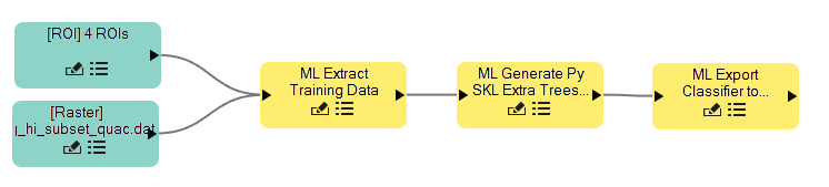
Using these tools, I was able to create an Extra Trees classifier which is an “extra random” version of random forest. Here is a link to a more detailed description: http://scikit-learn.org/stable/modules/ensemble.html#extremely-randomized-trees Extra trees performs quite well, is multi-threaded, and very easy to use (there are a whopping two parameters that you can tweak for your solution). One of the reasons that I love decision tree algorithms for image classification is that they require **no** iterations. A large part of neural networks is that you have to determine how many epochs or iterations that the classifier needs to be trained. This can take a very long time to train and may require lots of parameters tuning. Once I decided on the algorithm I wanted to generate, I used the ENVI Task API with IDL to extract tasks that training data from regions of interest, create a classifier, and classify the raster. For the classifier generation, here is what the simple workflow in the ENVI Modeler looks like which has steps 1 + 2 from the list above:

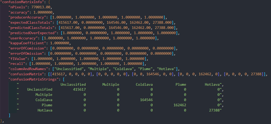
Once the workflow finishes running, we have two outputs: a classifier and a JSON file with a description of our classifier including metrics on our accuracy for the training data. For this example, there were 770,013 pixels in the training data. Amazingly enough, the extra trees classifier classified **every single pixel correctly**. Here is a look at the confusion matrix information which shows how well it performed:

Now that the classifier is generated, all that we need to do is then classify the original raster which uses a single ENVI Task. In total, for this scene, it took about 10 minutes to classify the image on my machine which was about 2.8 GB. Once classified, we are not quite done with our workflow. Instead, we are going to take it one step further and extract some meaningful information from our results. Specifically, we will create a proximity map for distance to the lava plume (volcanic gas). To accomplish this, you use the buffer zone task (new to ENVI 5.5.1) and a raster color slice to extract distance information. The end results for the classification and the proximity map then look like this:

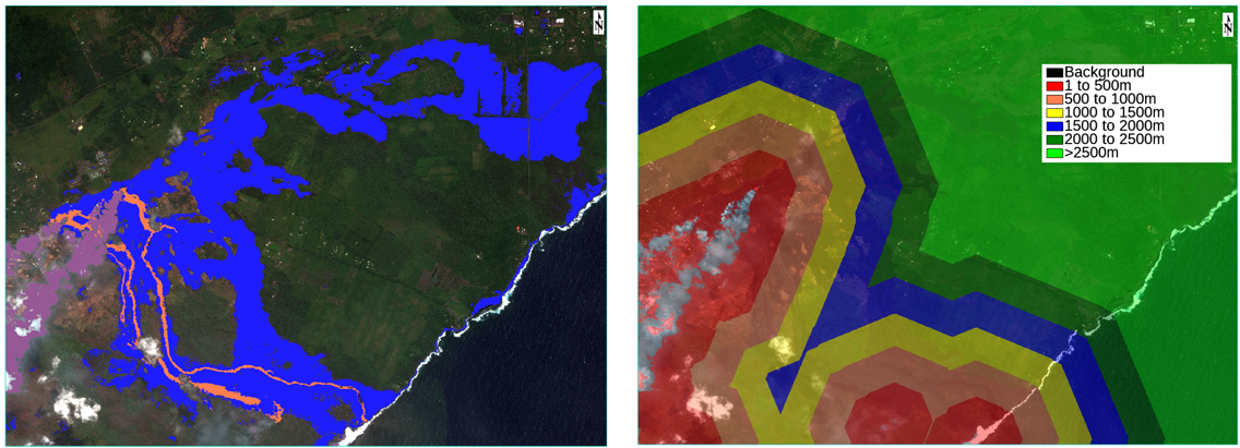
If you look at the classification result on the left, you can see that it did a very good job at extracting our features. About the only area that could be improved (might not work) would be trying to extract the areas where the plume is not as thick as you can see through it. One thing that is worth pointing out is that the classifier was able to delineate between the clouds and the plume which shows that they are spectrally different from one another.

Enjoy!