Accessing Features Only Available to 32-bit IDL from 64-bit IDL
Not all functionality available to IDL and ENVI in 32-bit mode is available in 64-bit mode, and vice versa.
There are multiple tables in our online documentation that list support for various platforms.
If you're on a 64-bit platform, you have the option of launching IDL in either 32- or 64-bit mode. But that doesn't really solve the problem.
For example, let's say you have a main application that executes in 64-bit IDL, but you want to have access to data in DXF-format files. If you attempt to create an instance of an IDLffDXF object that parses this file format, you'll get an error:
IDL> heart = obj_new('idlffdxf', filepath('heart.dxf', subdir = ['data']))
% OBJ_NEW: Dynamically loadable module is unavailable on this platform: DXF.
% Execution halted at: $MAIN$
We could fire up a second command line or Workbench session of IDL in 32-bit to parse the file, but a more convenient method, and the way we would want to implement a solution within a compiled routine, is through an IDL_IDLBridge object. There's a special keyword named OPS (technically, "out-of-process server") which allows us to set whether the bridge process should run in 32- or 64-bit mode.
Here, we'll start a 32-bit IDL process from our 64-bit IDL session.
IDL> b = idl_idlbridge(ops = 32)
% Loaded DLM: IDL_IDLBRIDGE.
Obviously, if you're on a 32-bit platform (still?!) you cannot simply create a 64-bit process via the magic of an IDL keyword.
We can construct a command to be executed in our 32-bit process to read the data.
IDL> command = "heart = obj_new('idlffdxf', filepath('heart.dxf', subdir = ['examples','data']))"
IDL> b->execute, command
Now we can proceed with an example from the documentation for the IDLffDXF::GetEntity method's documentation, transferring the data back to our main process for display.
IDL> b->execute,  "heartTypes = heart->getcontents()"
IDL> b->execute, "tissue = heart->getentity(heartTypes[1])"
IDL> b->execute, "connectivity = *tissue.connectivity"
IDL> b->execute, "vertices = *tissue.vertices"
IDL> vertices = b.getvar('vertices')
IDL> connectivity = b.getvar('connectivity')
Now that we have local copies in our 64-bit process of the vertices and connectivity list data from the 32-bit process, we can display the result.
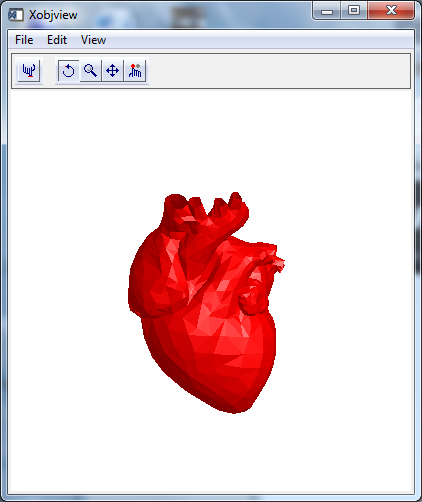
IDL> poly = idlgrpolygon(vertices, poly = connectivity, style = 2, color = !color.red)
IDL> xobjview, poly