Continuum Removal

Recently, I was given the chance to practice some spectroscopy and in preparation for the project, I realized that I did not have a simple way to visualize the variations in different absorption features between very discreet wavelengths. The method that I elected to employ for this task is called continuum removal  (Kokaly, Despain, Clark, & Livo, 2007). This method allows you to compare different spectra and essentially normalize the data so that they can be more easily compared with one another.

To use the algorithm, you first select the region that you are interested in (for me this was between 550 nm and 700 nm -this is the region of my spectra that deals with chlorophyll absorption and pigment). Once the region is selected then a linear model is fit between the two points and this is called the continuum. The continuum is the hypothetical background absorption feature, or artifact or other absorption feature, which acts as the baseline for the target features to be compared against (Clark, 1999). Once the continuum has been set then the continuum removal process can be performed on all spectra in question using the following equation (Kokaly, Despain, Clark, & Livo, 2007).

 R_C is the resulting continuum removed spectra, R_L is the continuum line and, R_o is the original reflectance value.

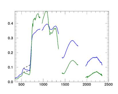
Figure 1: Original spectra of two healthy plants. The dotted line denotes the continuum line. The x axis shows wavelengths in nm and the y axis represents reflectance.

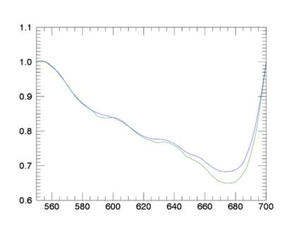
Figure 2: The continuum removal for wavelengths 550 nm - 700 nm.

 

The resulting code gives you a tool that will take in two spectral libraries, with one spectra per library, and return two plots similar to what is shown in Figure 1 and Figure 2.

 

pro Continuum_Removal

compile_opt IDL2

 

Spectra_File_1  =

Spectra_File_2 =

 

; Find the bounds for the feature

FB_left = 550

FB_right =700

 

; Open Spectra 1

oSLI1 = ENVISpectralLibrary(Spectra_File_1)

spectra_name = oSLI1.SPECTRA_NAMES

Spectra_Info_1 = oSLI1.GetSpectrum(spectra_name)

 

; Open Spectra 2

oSLI2 = ENVISpectralLibrary(Spectra_File_2)

spectra_name = oSLI2.SPECTRA_NAMES

Spectra_Info_2 = oSLI2.GetSpectrum(spectra_name)

 

; Get the wavelengths

wl = Spectra_Info_1.wavelengths

 

; Create Bad Bands List (this removes some regions of the spectra associated with water vapor absorption)

bb_range = [[926,970],[1350,1432],[1796,1972],[2349,2500]]

bbl = fltarr(n_elements(wl))+1

dims = size(bb_range, /DIMENSIONS)

for i = 0 , dims[1]-1 do begin

  range = bb_range[*,i]

  p1 = where(wl eq range[0])

  p2 = where(wl eq range[1])

  bbl[p1:p2] = !VALUES.F_Nan

endfor

 

;Plot oSLI1 / oSLI2

p = plot(wl, Spectra_Info_1.spectrum*bbl, xrange = [min(wl, /nan),max(wl, /nan)],$

  yrange=[0,max([Spectra_Info_1.spectrum*bbl,Spectra_Info_2.spectrum*bbl], /nan)], thick = 2, color = 'blue')

 

p = plot(wl, Spectra_Info_2.spectrum*bbl, /overplot, thick = 2, color = 'green')

 

; create the linear segment

Spectra_1_y1 = Spectra_Info_1.spectrum[where( wl eq FB_left)]

Spectra_1_y2 = Spectra_Info_1.spectrum[where( wl eq FB_right)]

pl_1 = POLYLINE([FB_left,FB_right], [Spectra_1_y1, Spectra_1_y2], /overplot, /data, thick = 2, LINESTYLE = '--')

Spectra_2_y1 = Spectra_Info_2.spectrum[where( wl eq FB_left)]

Spectra_2_y2 = Spectra_Info_2.spectrum[where( wl eq FB_right)]

pl_2 = POLYLINE([FB_left,FB_right], [Spectra_2_y1, Spectra_2_y2], /overplot, /data, thick = 2, LINESTYLE = '--')

 

; Get the equation of the line

LF_1 = LINFIT([FB_left,FB_right], [Spectra_1_y1, Spectra_1_y2])

LF_2 = LINFIT([FB_left,FB_right], [Spectra_2_y1, Spectra_2_y2])

 

; Get the values between the lower and upper bounds

x_vals = wl [ where(wl eq FB_left) : where(wl eq FB_right)]

 

; Compute the continuum line

RL_1 = LF_1[0] + LF_1[1]* x_vals

RL_2 = LF_2[0] + LF_2[1]* x_vals

 

; Perform Continuum Removal

Ro_1 = Spectra_Info_1.spectrum[ where(wl eq FB_left) : where(wl eq FB_right)]

RC_1 =  Ro_1 / RL_1

Ro_2 = Spectra_Info_2.spectrum[ where(wl eq FB_left) : where(wl eq FB_right)]

RC_2 = Ro_2 / RL_2

 

; Plot the new Continuum Removal Spectra

pl_RC_1 = plot(x_vals, RC_1, color = 'Blue', xrange = [min(x_vals, /NAN), max(x_vals, /NAN)] )

pl_RC_2 = plot(x_vals, RC_2, color = 'Green', /overplot)

 

end

 

Kokaly, R. F., Despain, D. G., Clark, R. N., & Livo, K. E. (2007). Spectral analysis of absorption features for mapping vegetation cover and microbial communities in Yellowstone National Park using AVIRIS data.

Clark, R. N. (1999). Spectroscopy of rocks and minerals, and principles of spectroscopy. Manual of remote sensing, 3, 3-58.