Using The Landsat 8 Quality Assessment Band
Anonym
The launch of Landsat 8 has been the talk of the remote sensing community for good reason. This not only continues NASA’s streak of constant earth observation since 1972, but this satellite brings something new to the scientific community, the Quality Assessment (QA) Band. According to the USGS Landsat Missions webpage, “Used effectively, QA bits improve the integrity of science investigations by indicating which pixels might be affected by instrument artifacts or subject to cloud contamination.” In short the QA Band lets the end user identify “bad” pixels more easily and single out the “good” data to produce more accurate and precise results. The utility of this new band can be taken in many directions, so we’ll tighten our focus on using it to differentiate urban areas from snow-packed areas, a constant problem encountered in the community. The thermal band present in previous and current Landsat satellites does have the ability to make this difference apparent, but what happens when the urban roofs are covered in snow? Things start to get more complicated! Well, step into that phone booth, strip off those glasses and suit, LDCM, because this is where the QA Band comes to the rescue!
Let’s take a look at the QA Band in the new ROI Tool in ENVI 5.1. Here is a grayscale view of the QA Band:
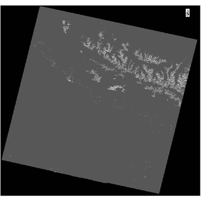
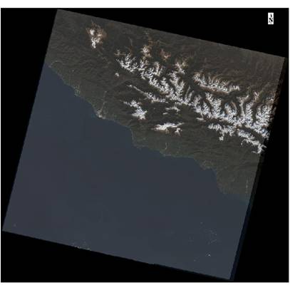
The lighter colors at the top-right of the image are actually the peaks of some mountains to the north of Sochi, Russia. Looking to the south of those peaks you can tell that some other bright colors are displayed. This is actually the coastline of the Black Sea. The following image shows a transparent view of the QA Band over a true color composite of the Landsat Data:
Now, let’s use this QA Band to extract the snow covered areas in the scene and avoid extracting the urban areas. We begin by applying Raster Color Slices to the QA Band to quickly identify which pixels are urban and which are snow. This Raster Color Slice image is a great start and through the use of the Cursor Value Tool we can identify many data ranges for snowpack:
Zooming in, we can see a clear difference in the color slice between the coastline and the snow covered peaks. Notice the red colors seen in the northeast corner of the image versus the light green and orange in the southwest along the coastline:
To hone in on the values of the snow you can look at the class ranges in the Layer Manager, and turn certain classes on an off until you can define specific ranges, or you can use the Cursor Value Tool to extract precise values of the snow covered peaks. Through a mixture of these two approaches we identified several values from the QA Band that indicate snow solely, and little to no urban areas. The values are noted because these will be our Band Thresholds applied within the ROI Tool. In the ROI Tool I select the Threshold tab, select Add New Threshold Rule, and choose the QA Band as the Input File. A Histogram is displayed showing the data values of the QA Band.
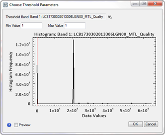
The spike in data values seen on the far left of the spectrum are the “no data” borders surrounding all Landsat images. We will use the data values found in the cursor value tool and the Raster Color Slice ranges to develop ROIs over the snow covered peaks. The Preview window allows the user to ensure they have chosen an appropriate threshold. The data values that we have found for snow cover are 23552, 31744, 39936 and 61440. Apply each thresholding to the new ‘Snow’ ROI and form a nearly complete capture of the snow found in the scene.
Once all of these classes are combined in the ‘Snow’ ROI, our display will show just how well we did capturing only the snowy peaks.
There you have it! Using the QA Band with ROI Band Thresholding has cut 25% of the time off this classification! This technique works not only for differentiating between snow covered mountains and highly-reflective urban areas, but for creating and separating all sorts of land cover types, all because of the QA band. The addition of the Quality Assessment Band has taken the great Landsat imagery product and made it even better, and easier to use. What will you be doing with it?