Hyperspectral Classification Workflows Integrating Dimensionality Expansion for Multispectral Imagery
Authors: Daniel C. Heinz, Thomas Bahr and Greg Terrie (NV5)
Many methods have been developed for target detection and classification in hyperspectral imagery. However, application of these methods to multispectral imagery presents a challenging problem due to a relatively low number of spectral bands available for analysis. Since a multispectral image may contain more targets than spectral bands, there may exist insufficient dimensionality to accommodate the proper classification of all targets in the image scene. To resolve this dilemma, a dimensionality expansion (DE) technique is introduced. These expanded bands ease the problem of insufficient bands in multispectral imagery and can improve and enhance the performance by exploiting band-to-band nonlinear correlation. In this paper, we utilize this DE to apply hyperspectral target detection and classification methods to multispectral imagery. A visual modelling tool is used to build multiple classification workflows using these hyperspectral target detection techniques and to incorporate the DE into the classification process.
- Index Terms
- Target detection, hyperspectral classification, dimensionality expansion, modelling tool, band number constraint
Introduction
This research demonstrates how hyperspectral classifiers can be effective at detecting and discriminating among targets using multispectral imagery, enhanced by Dimensionality Expansion (DE). Scene derived target endmember spectra are used with two standard supervised hyperspectral classifiers, the Adaptive Cosine/Coherence Estimator (ACE) and Matched Filter (MF). Visible Wildfire Airborne Sensor Program (WASP) data from Rochester Institute of Technology’s SpecTIR Hyperspectral Airborne Experiment (SHARE) data experiments is utilized [1]. This SHARE data is excellent for studying algorithm performance since ground truth is available for both the pure and mixed pixel targets.
A multispectral or hyperspectral image is often visualized as a three-dimensional dataset, where two of the dimensions are used to locate the spatial position of an image pixel and the third dimension specifies a spectral band. The classification of pure pixel targets and mixed pixel targets can be difficult due to the small number of spectral bands available in multispectral imagery. A multispectral sensor typically records less than 10 spectral bands, with spectral resolution of approximately 100 nm. In contrast, a hyperspectral sensor can acquire hundreds of bands with a spectral resolution on the order of 10 nm. It is this small number of spectral bands in multispectral data that presents a problem to subpixel and pure pixel target classification. This fact is similar to the well-known pigeon-hole principle in discrete mathematics [2].
To mitigate this lack of dimensionality a DE technique [3] was developed which makes use of various nonlinear transformations among the original multispectral bands to produce additional bands. Combining these newly generated bands with the original bands results in an increase of data dimensionality which helps improve the performance of linear target classification methods.
In this paper we selected target spectra directly from the target scene. The DE results in these target spectra becoming more unique. This target uniqueness works well for the targets and data scene presented in this paper. However, if targets exhibit significant spectral variability then a multiple target approach [4] or target subspace approach [5] or other approaches may be necessary [6].
The use of models made the process of testing these classifiers and comparing the results much more efficient, compared to writing API code or invoking tools through a user interface. Model nodes can be easily interchanged to accommodate different classifiers. Models can also be packaged and deployed to desktop and cloud-computing environments for reuse and further customization.
The remainder of this paper is organized as follows. Section 2 describes the DE method and Section 3 briefly describes a classification method. This is followed by Section 4 which describes a classification model. Sections 5 and 6 present experimental results and conclusions.
DIMENSIONALITY EXPANSION
The success of hyperspectral classification methods lies in the fact that there is sufficient data dimensionality to accommodate each distinct material to be classified. However, this may not be true for multispectral imagery where the number of materials may be greater than the number of bands. In this case, some of materials will be mixed and blended with other materials, which results in poor performance. In this section, we make use of a DE developed in [3] to expand dimensionality of the original multispectral image data.
The idea of a DE arises from the fact that a second-order random process is generally specified by its first order and second-order statistics. If we view the original bands as the first-order statistical images, we can then generate a set of second order statistical bands by capturing correlation between bands. These correlated images provide useful second-order statistical information about the bands, which is missing from the original set of bands. The desired second order statistics including autocorrelation, cross-correlation and nonlinear correlation can be used to create nonlinearly correlated images. The concept of producing second-order correlated bands coincides with that used to generate covariance functions for a random process.
CLASSIFICATION METHOD
Advanced spectral classifiers have been specifically developed for hyperspectral images, but they can also perform well on imagery with limited spectral resolution after DE transformation. For this study, two supervised classifiers, the Matched Filter (MF) and Adaptive Cosine/Coherence Estimator (ACE) were selected to assess the effectiveness of DE transformation against different target classification methods based on their best overall accuracies demonstrated in [7]. Matched Filtering [5] finds the abundance of targets using a partial unmixing algorithm. This technique maximizes the response of the known spectra and suppresses the response of the composite unknown background, therefore matching the known target signature. Responses from the MF can be both positive and negative and have magnitudes greater than one. ACE [5] is derived from the Generalized Likelihood Ratio (GLR) approach, based on the assumption that the background covariance matrix is known. It is invariant to relative scaling of test and training data and has a Constant False Alarm Rate (CFAR) with respect to such scaling. ACE uses a different way to stretch the detection statistic and to achieve greater target to background separation. Responses from the ACE detector range from zero to one.
CLASSIFICATION MODEL
Classification models were built using the ENVI® 5.6 Modeler for the MF and ACE classifiers with and without DE. These models were simple to construct as they all had the same basic elements, except for the DE transformation. Figure 1 shows an example of the ACE model.
The models consist of yellow-coloured nodes that represent individual tasks as well as operations that act upon the data (such as querying the spectral library). Nodes can be selected from a list of available tasks and data-processing operations, then dragged and dropped into a canvas to build a model. Nodes are connected so that input and output parameters can be passed from one task to another.
The first part of a classification model (Figure 1a) includes steps to prepare the input raster data for classification. The Input Parameters node displays a dialog for the user to select an input image, an input ROI, and a spectral library with reference spectra from data regions of interest (ROIs). ROI Subsetting opens a ROI, creates an array of subrects based on this ROI, and subsets the input raster file spatially. The Raster Normalization tasks extract the individual bands from the WASP data, scale the original data values from 1 to 2 (band-wise in combination with the upstream loop iterator), and stack the bands into one raster using an upstream aggregator node to build an array of input bands. Finally, Dimensionality Expansion Raster is an interchangeable element to increase the multispectral data dimensionality of the input raster data.
The next part of the model (Figure 1b, left) completes the steps for preparing the reference spectra for classification. Dimensionality Expansion SLI is used here to increase the data dimensionality of the input spectral library to match with the DE bands of the raster data. Query Spectral Library queries the input spectral library, returning the names of all spectra in the library. In combination with the upstream Iterator, Get Spectrum from Library retrieves in a loop each reference spectrum and its metadata.
Figure 1b shows the last remaining nodes in the model for Classification and Output. The Adaptive Coherence Estimator node performs the actual classification. The Generate Filename node allows to specify filenames (including iteration indices from the Iterator node) and locations for the classification task output. The Aggregator node collects the multiple classification results (i.e., one rule-image for each reference spectrum) and passes them to the Build Band Stack node to build the final classification raster. The Output Parameters node ensures that model users can access the output.
When the model runs, it writes the classification raster to disk. The result contains a series of grayscale bands, one for each endmember (so-called rule images).
Fig. 1a.Nodes for preparing input raster data in the classification models. The red box denotes the interchangeable element for DE.
Fig. 1b. Nodes for preparing input reference spectra in the classification models, for classifying the raster (here: ACE) and for preparing output data. The red boxes denote the interchangeable elements for DE and the classifier.
EXPERIMENTAL RESULTS
Three band RGB visible WASP data from Rochester Institute of Technology’s SHARE data experiments [1] was used for image classification. The image was acquired during the 2012 data experiments with a spatial resolution of 0.1 m.
The following processing steps were used with ENVI® 5.6 software to prepare the image for analysis:
- Defining a spatial subset around the area of interest.
- Using the Band Algebra/Band Math to scale the original data values from 1 to 2.
- Applying the DE tool to the scaled data to generate nonlinearly correlated spectral band images.
- Using the ROI tool to select six target endmember spectra from the image scene: “Pink Felt”, “Yellow Cotton”, “Yellow Felt”, “Blue Cotton”, “Gold Felt” and “Blue Felt”.
- Selecting compute statistics from ROI tool and export the mean target spectra in a spectral library.
- Using the Spectral Math to scale the mean target spectra values from 1 to 2.
- Using the scaled mean target spectra as the target for the ACE (ACE classification tool and with the Y multiplier set to 1.0) and MF classification tools.
The resulting dataset contains 15 spectral bands, listed in Table 1. Bands B1 to B3 correspond to the scaled original multispectral bands of the WASP image product. Table 1 includes the formulas used for the computation of bands B4 to B15. The DE used to generate the fifteen bands were selected empirically based on observed performance results. Methods to optimize this selection remain an ongoing work.
Figure 2 shows a true color RGB composite image of the region of interest considered in this paper. The target set included six 10’ x 10’ solid panels: “Pink Felt” and “Yellow Cotton” in one row (left to right) and “Yellow Felt”, “Blue Cotton”, “Gold Felt” and “Blue Felt” in the second row (left to right)). Additionally, there were two checkboard targets each consisting of 12”x12” squares in a repeating pattern. One was a 16’ x 16’ panel was made with a 2x2 repeating pattern comprised of 3 “Yellow Felt” squares and 1 “Yellow Cotton” square, thus achieving a 75%/25% area fraction. The second was a larger (24’ x 24’) 50%/50% mixture of “Blue Cotton” and “Blue Felt” squares [8].
Table 2 contains results for ACE and MF classification with and without DE for the pure and mixed yellow felt target. Typically, it is desired that a detector will provide output values close to zero when no target is present and values greater than zero when the target is present. Determining thresholds for classification can be difficult.
Tab. 1.WASP spectral bands (B1-B3) and associated dimensionality expansion.
| Band Number |
Band Name |
| B1-B13 |
Red, Green, Blue |
| B4-B6 |
B1*B2, B1*B3, B2*B3 |
| B7-B9 |
B1/B2, B1/B3, B2/B3 |
| B10-B12 |
B2/B1, B3/B1, B3/B2 |
| B13-B15 |
B1^2, B2^2, B3^2 |
Fig. 2. Test site with six pure fabric targets and two checkerboard mixed fabric targets.
For all experiments a threshold of 0.1 was used to indicate a detection for classification. This value worked well with DE, but without DE a much higher value is needed since many of the pixels resulted in large detector outputs. All the detectors except the ACE with DE correctly classified the pure target with a 100% Probability of Detection (PD), but the ACE with DE had the best performance for the mixed target. Figure 3a shows the results for the ACE with DE in which it correctly classified most of the pure target pixels in both the pure and checkerboard targets. Figure 3b shows results for ACE with no DE with many false alarms (Probability of False alarm, PFA).
Table 3 contains results for ACE and MF classification with and without DE for the pure and mixed yellow cotton target. As with the yellow felt the ACE detector with DE had the best performance for the mixed target. Figure 3c shows the results for the ACE with DE in which it correctly classified most of the pure target pixels in both the pure and checkerboard targets. Figure 3d shows results for ACE with no DE with many false alarms.
Table 4 contains results for ACE and MF classification with and without DE for the pure and mixed blue cotton target. All the detectors correctly classified the pure target with a 100% PD, but the ACE with DE had the best performance for the mixed target. Figure 3e shows the results for the ACE with DE in which it correctly classified most of the pure target pixels in both the pure and checkerboard targets. Figure 3f shows results for ACE with no DE with false alarms to the white tarp.
Table 5 contains results for ACE and MF classification with and without DE for the pure and mixed blue felt target. All the methods had difficulty with this target. The MF detector with DE had the best PFA performance. Figure 3g shows the results for the MF with DE in which it performed the best but detected many incorrect targets. A higher threshold for this target would help, but not completely solve this issue. Figure 3h shows results for MF with no DE with false alarms to the white tarp, pink felt and blue cotton.
REFERENCES
[1] A. Giannandrea et al., “The SHARE 2012 Data Collection Campaign,” Proc. SPIE 8743, Baltimore, MD, USA, pp. 87430F1-87430F15, May 2013.
[2] Epp. S.S., Discrete Mathematics with Application, 2nd ed., Brooks/Cole Publishing, Pacific Grove, CA, USA, 1995.
[3] H. Ren and C.-I. Chang, “A Generalized Orthogonal Subspace Approach to Unsupervised Multispectral Image Classification,” IEEE TGRS 38/6, pp. 2515-2528, Nov 2000.
[4] C.-I. Chang and H. Ren, "LCMV beamforming approach to target detection and classification for hyperspectral imagery,” IGARSS, Hamburg, Germany, pp. 1241-1243, vol.2, 1999.
[5] D. Manolakis, et al., “Hyperspectral Image Processing for Automatic Target Detection Applications,” Lincoln Laboratory Journal 14/1, Lexington, MA, USA, pp. 79-116, 2003.
[6] D. Hong, et al., "An Augmented Linear Mixing Model to Address Spectral Variability for Hyperspectral Unmixing," IEEE TIP 28/4, pp. 1923-1938, April 2019.
[7] T. Bahr and D.C. Heinz, “Creating Models of Hyperspectral Classification Workflows Integrating Dimensionality Expansion for Multispectral Imagery,” WHISPERS, Amsterdam, Sept. 2019.
[8] J.P. Kerekes, et al.,” SHARE 2012: Subpixel Detection and Unmixing Experiments,” Proc. SPIE 8743/87430H, Baltimore, MD, USA, pp. 87430H1-87430H15, May 2013.
Tab. 2. PD and PFA for yellow felt for ACE and MF with and without DE, thresholded at 0.1.
| Yellow Felt |
PD Pure |
PD Mixed |
PFA |
| Truth |
100% |
75% |
0% |
| ACE |
100% |
100% |
39.72% |
| MF |
100% |
100% |
1.53% |
| ACE & DE |
95.32% |
84.12% |
0.002% |
| MF & DE |
100% |
96.84% |
0.59% |
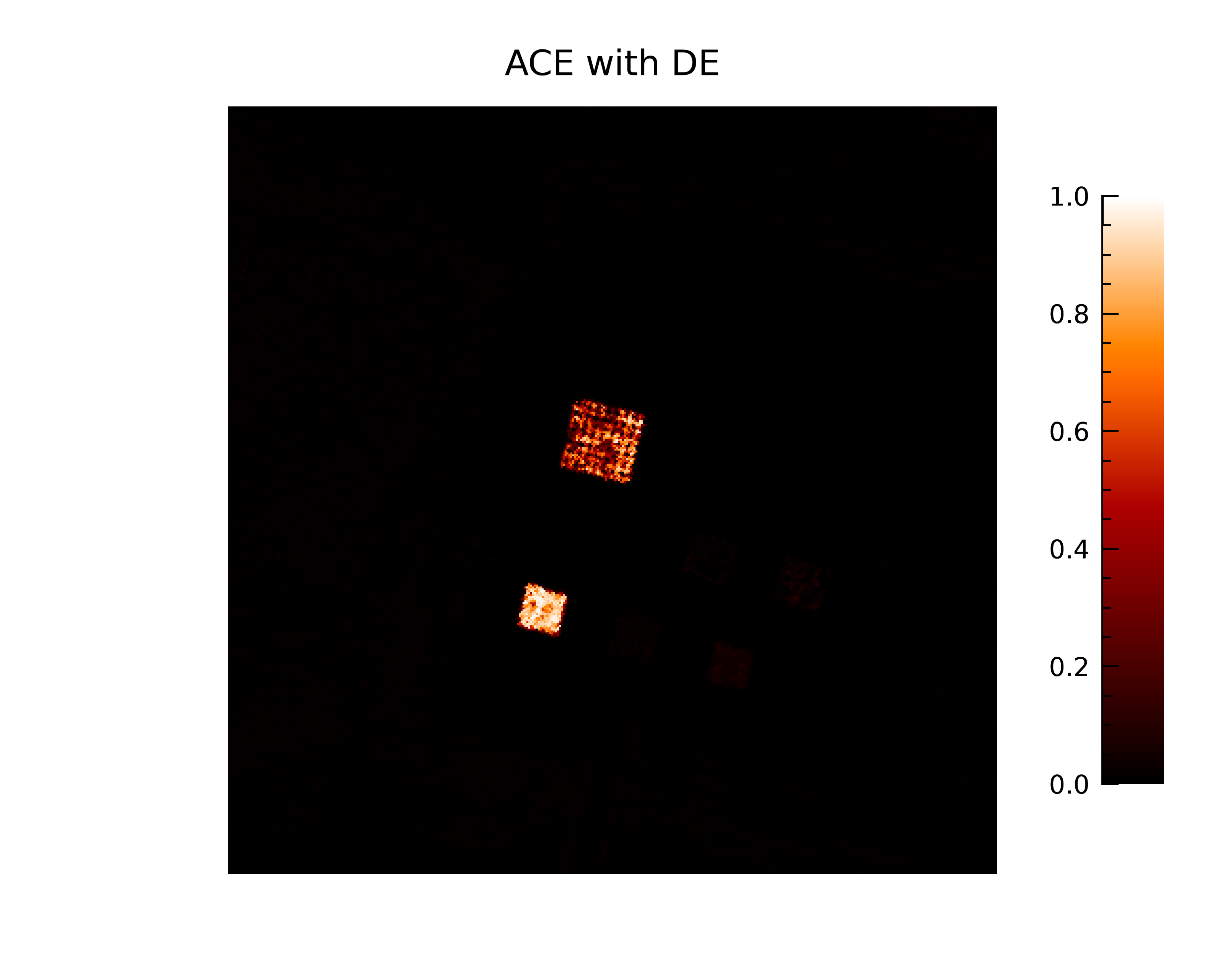 Fig. 3a. ACE with DE classification for pure and mixed yellow felt.
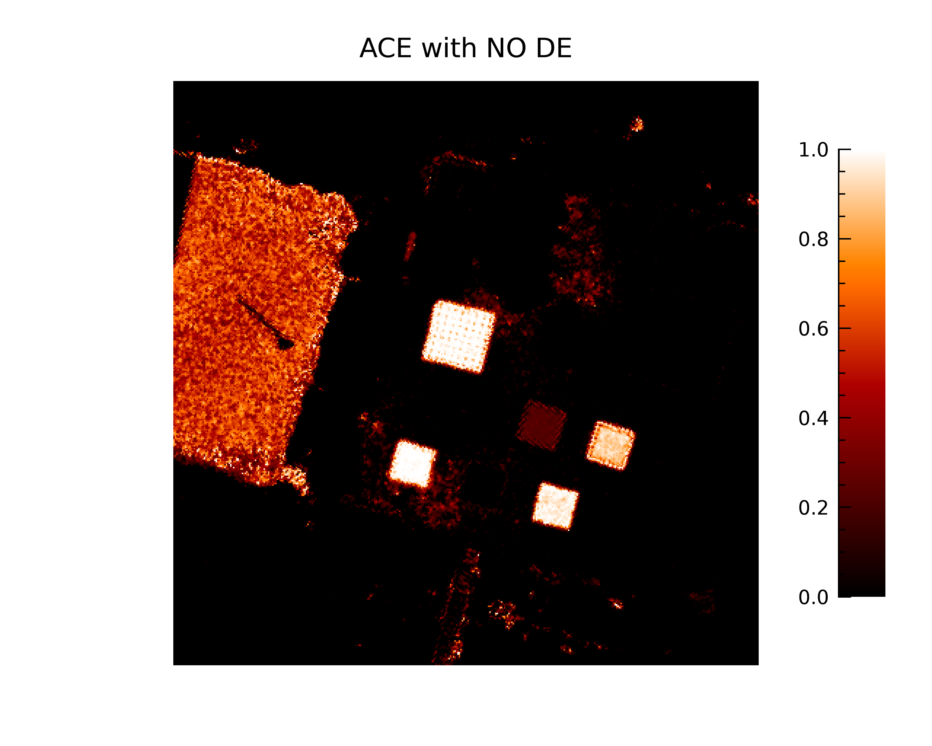 Fig. 3b.ACE with no DE classification for pure and mixed yellow felt.
Tab. 3. PD and PFA for yellow cotton for ACE and MF with and without DE, thresholded at 0.1.
| Yellow Cotton |
PD Pure |
PD Mixed |
PFA |
| Truth |
100% |
25% |
0% |
| ACE |
100% |
100% |
47.67% |
| MF |
100% |
100% |
1.33% |
| ACE & DE |
97.89% |
22.21% |
0.01% |
| MF & DE |
98.94% |
45.49% |
0.05% |
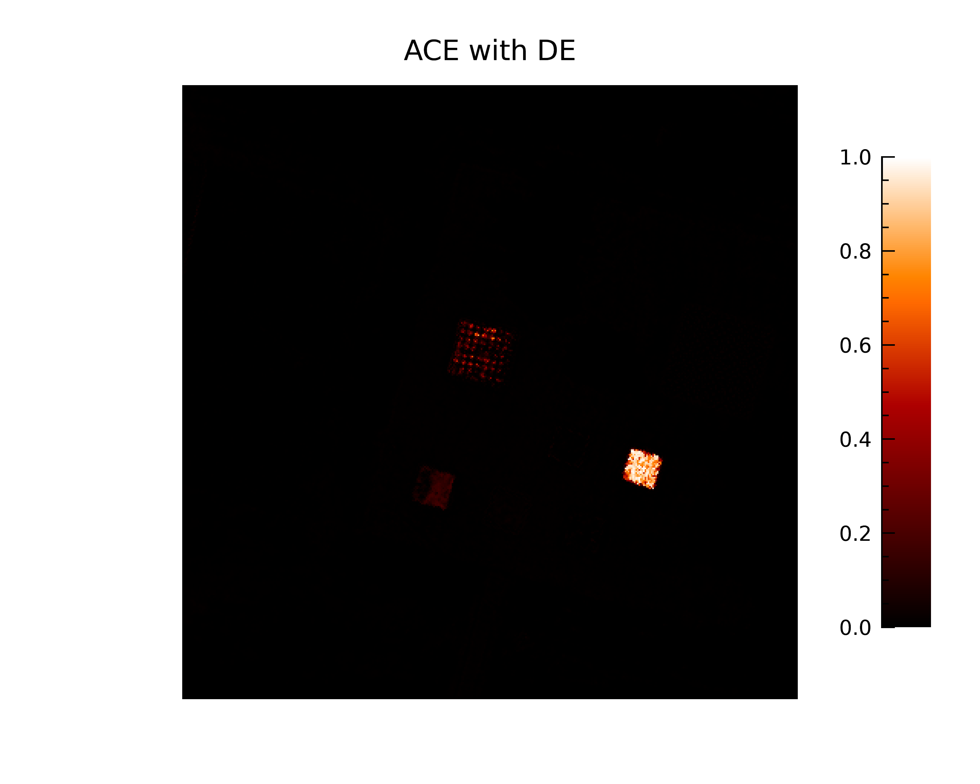 Fig. 3c. ACE with DE classification for pure and mixed yellow cotton.
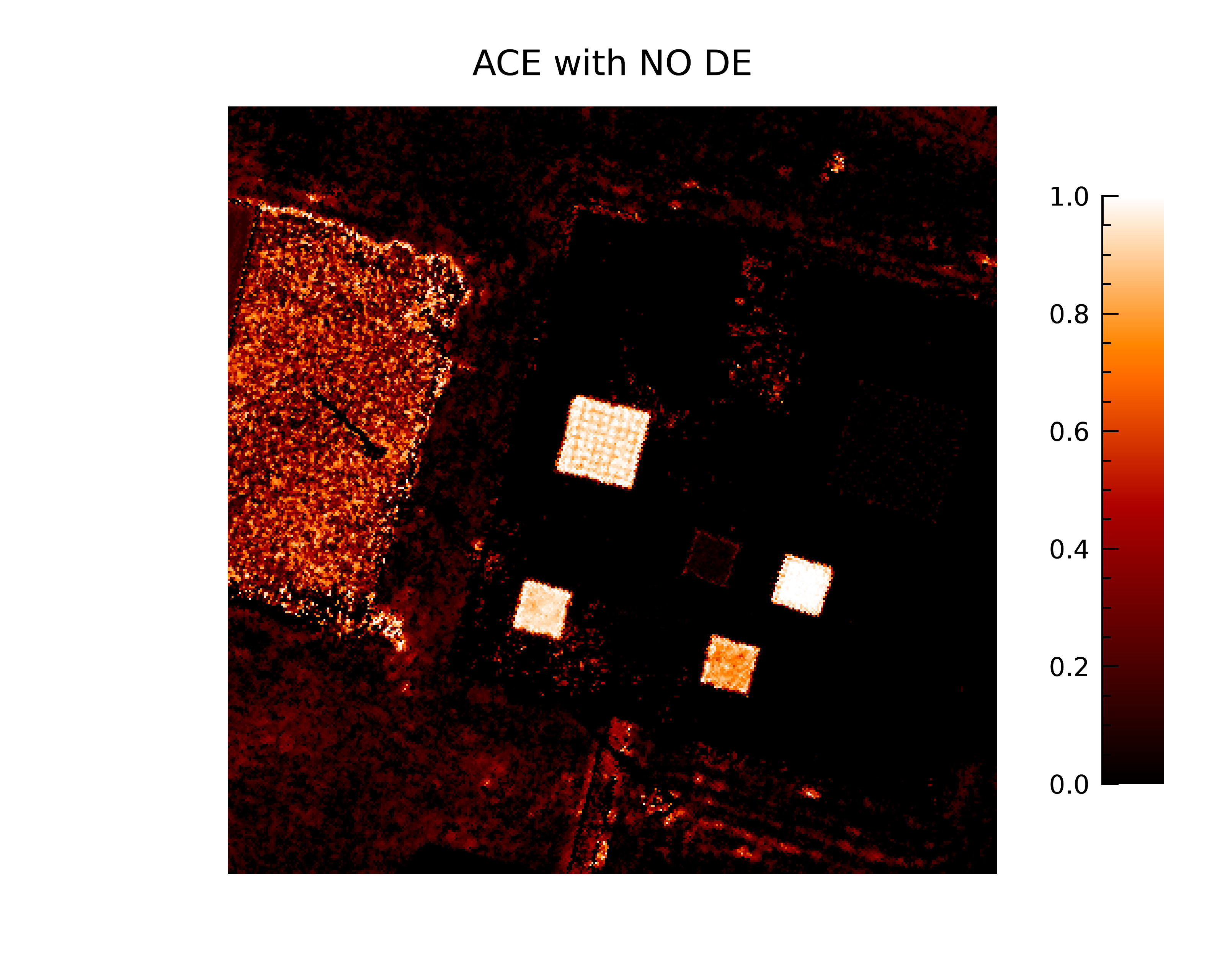 Fig. 3d. ACE with no DE classification for pure and mixed yellow cotton.
Tab. 4. PD and PFA for blue cotton for ACE and MF with and without DE, thresholded at 0.1.
| Blue Cotton |
PD Pure |
PD Mixed |
PFA |
| Truth |
100% |
50% |
0% |
| ACE |
100% |
95.73% |
36.1% |
| MF |
100% |
97.44% |
1.53% |
| ACE & DE |
100% |
60.672% |
0.05% |
| MF & DE |
100% |
77.39% |
0.547% |
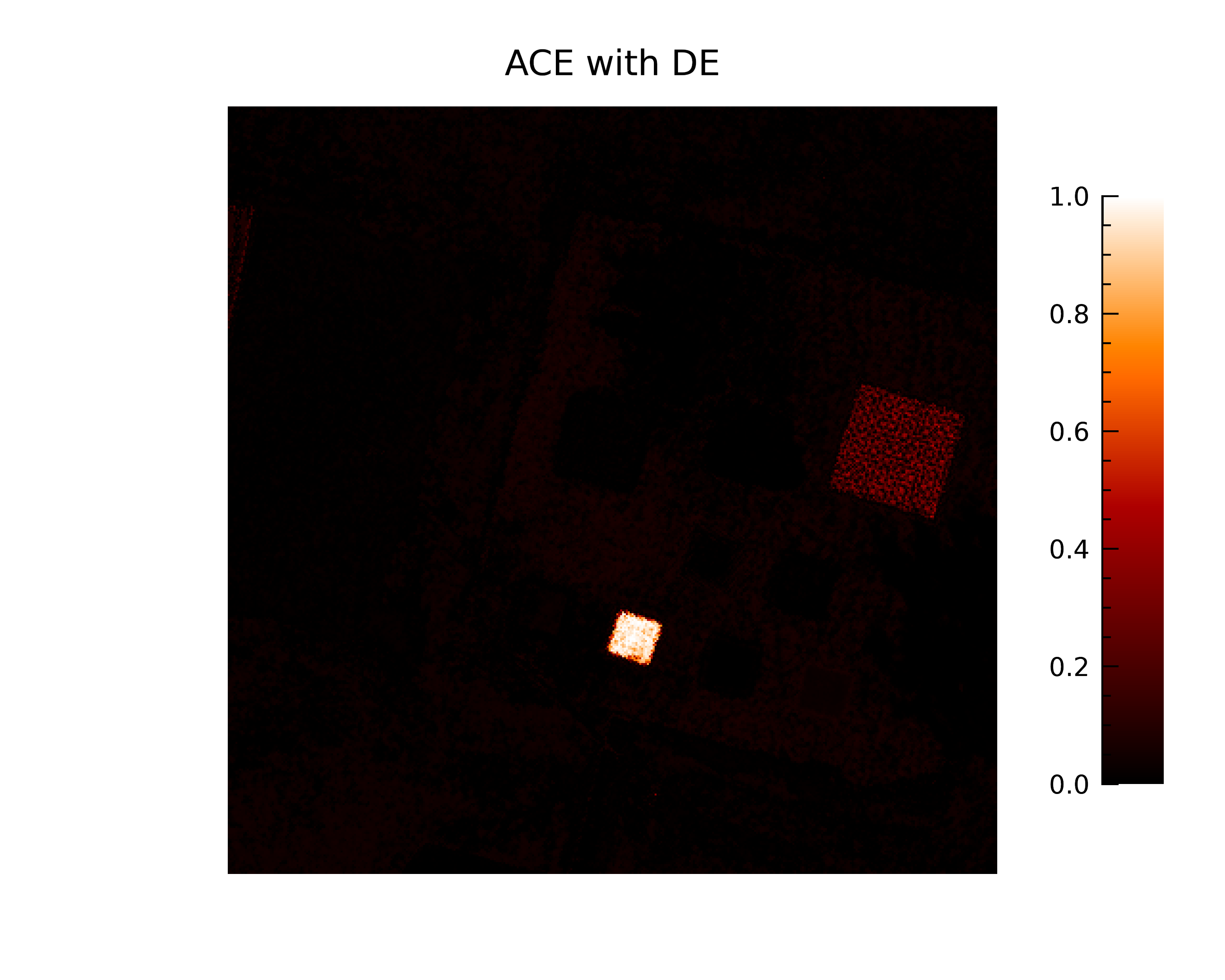 Fig. 3e. ACE with DE classification for pure and mixed blue cotton.
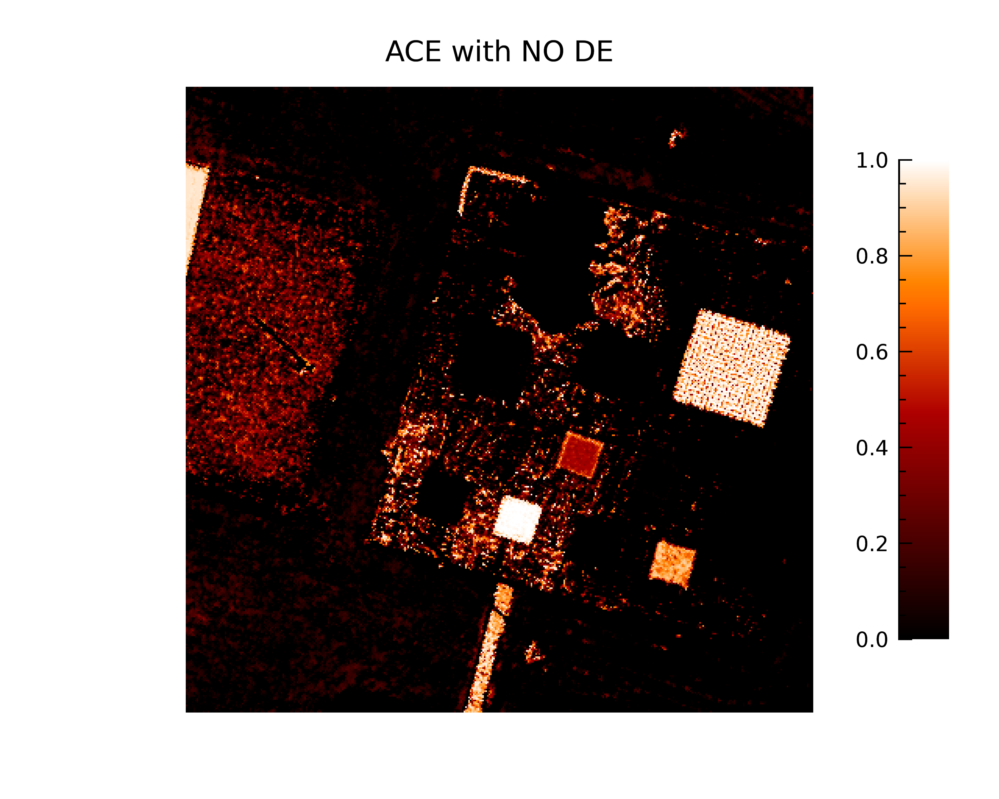 Fig. 3f.ACE with no DE classification for pure and mixed blue cotton.
Tab. 5. PD and PFA for blue felt for ACE and MF with and without DE, thresholded at 0.1.
| Blue Felt |
PD Pure |
PD Mixed |
PFA |
| Truth |
100% |
50% |
0% |
| ACE |
100% |
94.75% |
72.95% |
| MF |
100% |
99.97% |
39.95% |
| ACE & DE |
100% |
79.522% |
36.70% |
| MF & DE |
100% |
93.09% |
13.57% |
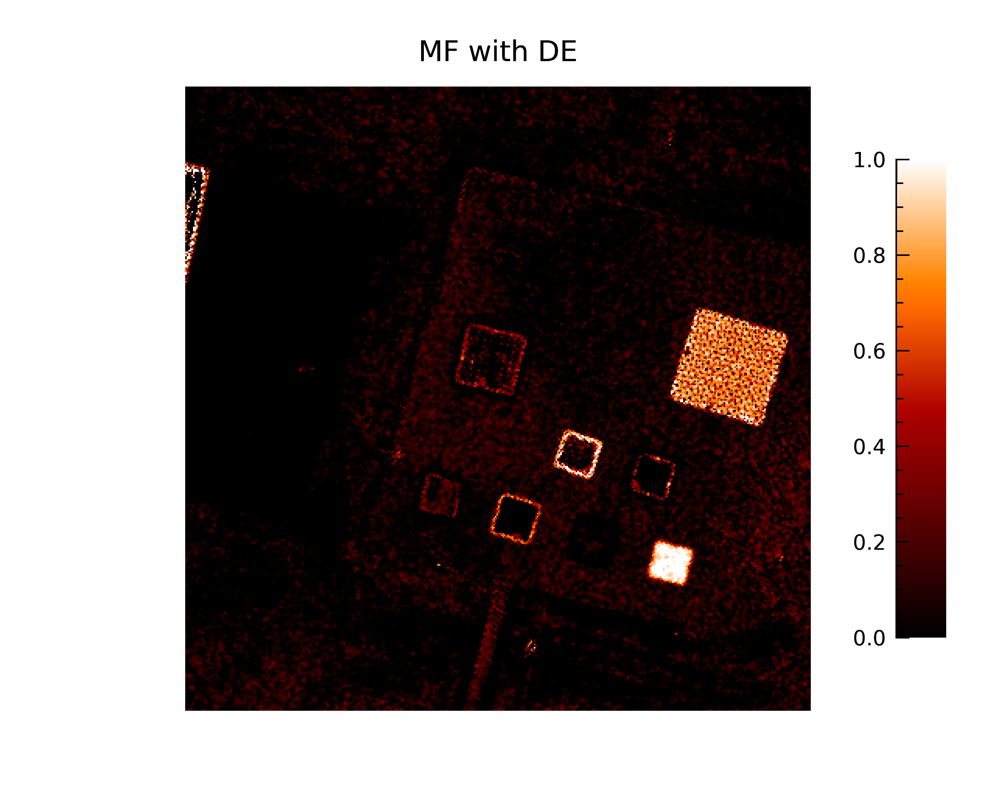 Fig. 3g. MF with DE classification for pure and mixed blue felt, range = [0,1].
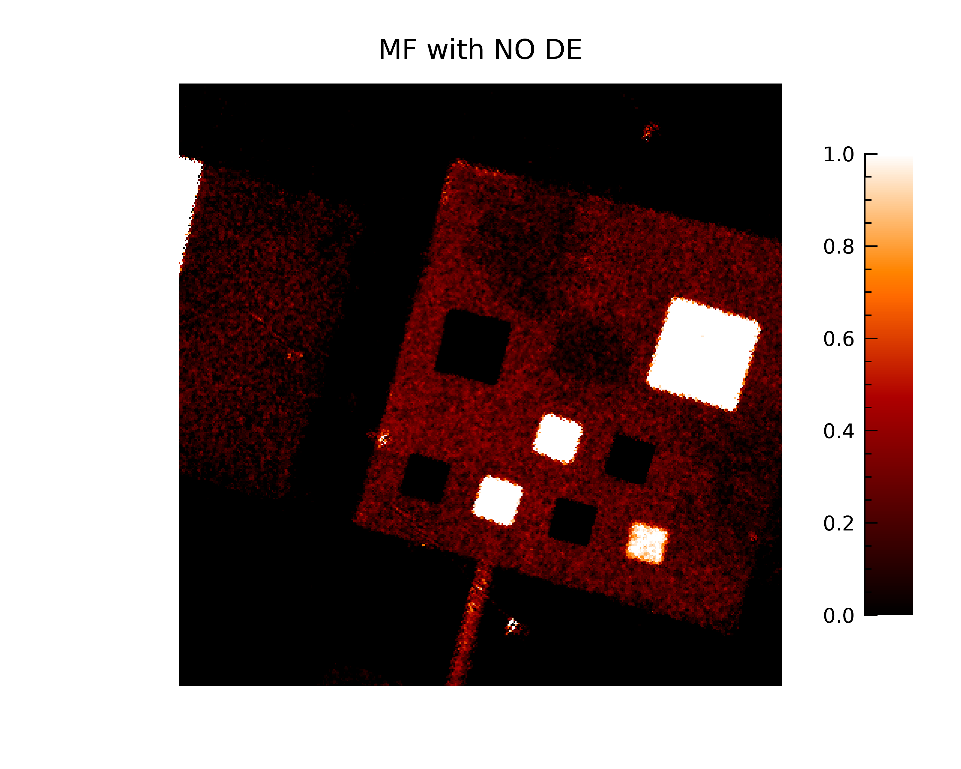 Fig. 3h.MF with no DE classification for pure and mixed blue felt, range = [0,1].