Combining IDL and Python Graphics

With the introduction of the Python bridge to IDL in 8.5, IDL and Python and graphics can coexist, but they do not live in the "same space".

You can't manipulate the contents of an IDL graphics scene within the context of a Python pyplot, for example.

However if either the Python or IDL scene is static, it's possible to capture the bitmap contents of the scene in one rendering context and apply it to the context of the other.

In the following example, I will show how to capture graphics from Python and embed them in IDL, then vice versa.

The following example has been adapted from the pyplot tuorial for the "hist" routine with some extra IDL magic thrown in.

I will show a technique to:

1. Generate example data and a histogram plot in Python, called from IDL
2. Copy the graphic from Python to IDL
3. Fit the data generated in Python within IDL to a Gaussian
4. Combine the Python graphic with IDL graphics into an IDL 3D view
5. Transfer the IDL graphic back to Python
6. Display the combined graphic in a new Python plot

We will use two Python modules in this example, matplotlib.pyplot and numpy. For the former, we will want to have references to the module in both IDL and Python. For the latter we only need a reference within Python since we don't access its functionality directly in IDL.

For those of you who like to know where we're going before we get there, copy and paste the following to your IDL command line.

; We'll need a reference to the pyplot on both the IDL and Python side.
plt = Python.Import('matplotlib.pyplot')
Python.plt = plt
plt.xkcd(scale=1,length=100,randomness=2)
; Generate some normally distributed sample data
Python.Run('import numpy as np')
Python.Run, 'mu, sigma = 100, 15'
Python.Run, 'x = mu + sigma * np.random.randn(10000)'
; the histogram of the data
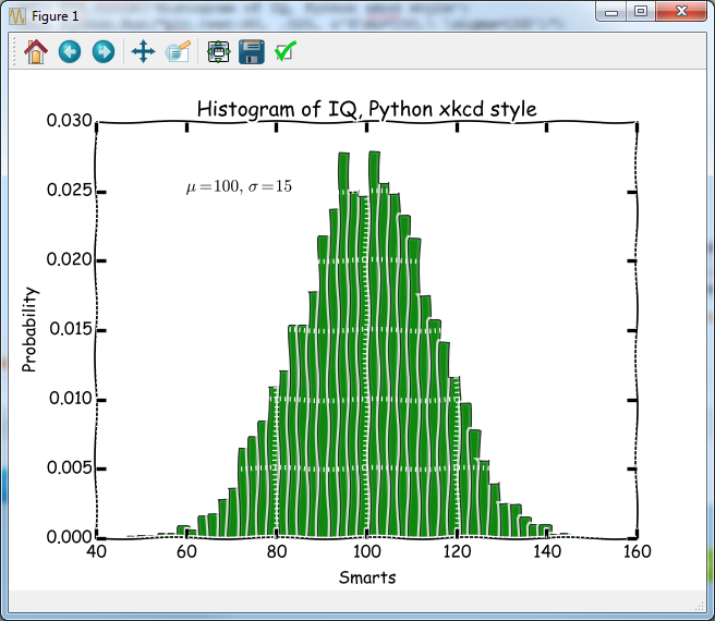
Python.Run, 'n, bins, patches = plt.hist(x, 50, normed=1, facecolor="g", alpha=0.75)'
plt.xlabel('Smarts')
plt.ylabel('Probability')
plt.title('Histogram of IQ, Python xkcd style')
Python.Run("plt.text(60, .025, r'$\mu=100,\ \sigma=15$')")
plt.axis([40, 160, 0, 0.03])
plt.grid(!true)
plt.show(!false)
file = filepath(/tmp, 'xkcd_plot.png')
plt.savefig(file) ; screen grab of the Python window
pyimage = read_png(file)
file_delete, file
; Python returns histogram bins as bin edges rather than centers.
; Convert to centers.
IDLbins = Python.bins
bins = (IDLbins[0:*] + IDLbins[1:*])/2
yfit = gaussfit(bins, Python.n, coeff)
i = image(pyimage, image_location = [20.5, -0.0038], image_dimensions = [155,  .0375], $
  aspect_ratio = 155/.0375, zvalue = -.01, clip = 0, dimensions = [1024, 768])
p = plot(bins, Python.n, xrange = [40, 160], yrange = [0, .030], /stairstep, $
  color = [0, 0, 255], thick = 2, clip = 0, /overplot)
p2 = plot(/overplot, bins, yfit, thick = 4, linestyle = 2, color = [0, 125, 0], clip = 0)
t = text(110, .025, 0, ['IDL Gaussfit Coefficients', '        ' + (String(coeff, format  = '(g11.4)')).Trim()], color = [0, 125, 0], /Data, /Onglass)
p.rotate, /reset
p.rotate, 25, /yaxis
p.rotate, 5, /xaxis
plt.close()
plt.rcdefaults()
shot = reverse(i.copywindow(), 3) ; Screen grab of the IDL image window
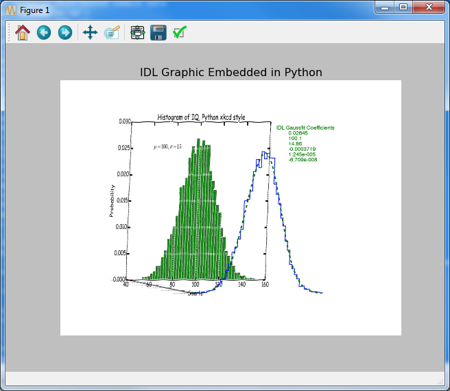
plt.title('IDL Graphic Embedded in Python')
plt.axis('off')
plt.imshow(shot) ; Show the IDL screen grab as an image
!null = plt.show(!false)

The end product of the above code is the following combined graphic:

First, create the reference to the "pyplot" module in IDL. We will use this reference within the IDL syntax.

IDL> plt = Python.Import('matplotlib.pyplot')

Next, we want to transfer the reference to this object from IDL back to Python. Accessing or setting a Python variable by name from IDL is as simple as specifying

IDL> IDL_variable = Python.name-in-python-scope

or

IDL> Python.name-in-python-scope = IDL_variable or expression

For this step we simply create a variable named "plt" in the Python context.

IDL> Python.plt = plt

In this example we've set the Python and IDL variable names to be identical, "plt", but there is no requirement that this must be so.

Because we only need the numpy module on the Python side, we can import it through a Python.Run function call directly.  This creates a variable named "np" on the Python side, but there's no equivalent on the IDL side.

IDL> Python.Run('import numpy as np')

[Note: You may notice that some output was emitted to the IDL console after executing this statement.  We're calling a Python function and it's returning a value. But for the sake of code simplicity I'm not capturing the output to a variable.  IDL will print the return value to the console in this case.]

I'm going to introduce a little bling to our Python plot.  I'll leave it to the reader to determine what this does!

IDL> plt.xkcd(scale=1,length=100,randomness=2)

Generate some normally distributed data on the Python side, and create its histogram distribution using the matplotlib functionality. This code comes from the matplotlib tutorial.

IDL> Python.Run('import numpy as np') IDL> Python.Run, 'mu, sigma = 100, 15' 
IDL>Python.Run, 'x = mu + sigma * np.random.randn(10000)'
IDL> Python.Run, 'n, bins, patches = plt.hist(x, 50, normed=1, facecolor="g", alpha=0.75)' 

Notice that the Python-side reference to "plt" is used in the fourth statement when its "hist" method is called.

Sometimes the syntax of Python requires us to execute the function Python.Run, as in the call to "plt.hist", above. There is no equivalent syntax for returning three different data types from a single IDL function call.

But we often have more than one other syntax option when using the Python bridge. For example, in the second and third statements above we could have also issued the following equivalent commands.

IDL> Python.mu = 100
IDL> Python.sigma = 15
IDL> Python.x = Python.mu + Python.sigma * Python.np.random.randn(10000)

As a general rule of thumb, it will be more efficient to leave variables on one side of the bridge or the other that aren't going to be shared between the environments.

Generate the axis labels and title for the plot.

IDL> plt.xlabel('Smarts')
IDL> plt.ylabel('Probability')
IDL> plt.title('Histogram of IQ, Python xkcd style')
IDL> Python.Run("plt.text(60, .025, r'$\mu=100,\ \sigma=15$')")
IDL> plt.axis([40, 160, 0, 0.03])
IDL> plt.grid(!true)

Show the result

IDL> plt.show(!false)

This statement will pop up a Python plot window.

I want to get a copy of this graphic, as-is, and move it to IDL for further manipulation.

A simple technique is to save the graphic to a temporary file from Python into a standard image format, in this case PNG, then read the image data from file into IDL.

IDL> file = filepath(/tmp, 'xkcd_plot.png')
IDL> plt.savefig(file)
IDL> pyimage = read_png(file)
IDL> file_delete, file

Be aware at this point that we've captured a bitmap representation of the Python graphic. It contains no information about font sizes, text element locations, or any of the other metadata that would allow us to smoothly scale the elements via any operation other than interpolation of the flat bitmap. Text elements in your graphics will not be re-rendered at a new font size, for example, if the destination window is enlarged or reduced, or if its aspect ratio changes.

Before including this graphic in an IDL scene, we'll perform simple analysis in IDL on the data that we created on the Python side. How well does the generated Python data fit the normalized distribution it claims to have created?

Python's histogram function "hist" returns the edges of the bins rather than the centers, so we first want to convert from edges to centers before executing IDL's GAUSSFIT function.

IDL> IDLbins = Python.bins
IDL> bins = (IDLbins[0:*] + IDLbins[1:*])/2
IDL> yfit = gaussfit(bins, Python.n, coeff)

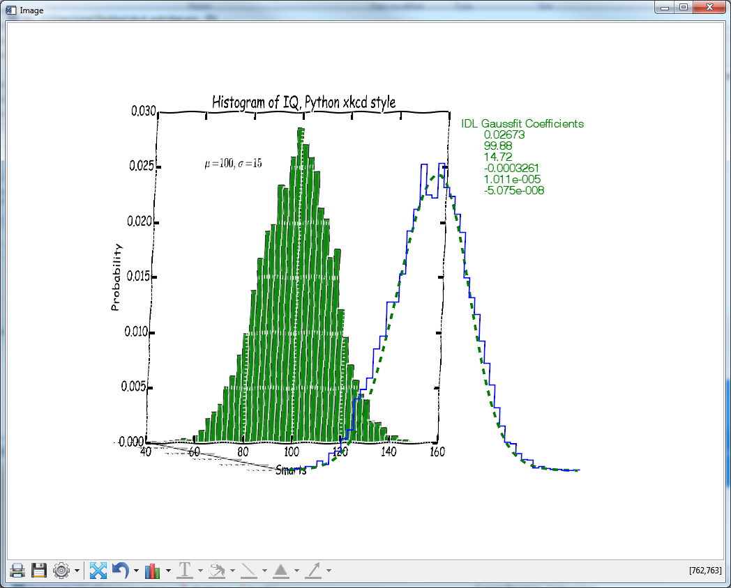
Display the Python histogram graphic as an IMAGE in the context of IDL.

IDL> i = image(pyimage, image_location = [20.5, -0.0038], $
IDL> image_dimensions = [155,  .0375], $
IDL> aspect_ratio = 155/.0375, zvalue = -.01, $
IDL>  clip = 0, dimensions = [1024, 768])

There are indeed some magic numbers in the IMAGE_LOCATION, IMAGE_DIMENSIONS, and ASPECT_RATIO keywords. How those may be determined is left as an exercise for the reader.

Overlay a PLOT of the histogram data. This is at a Z location closer to the eye than the image, which lies in the background.

IDL> p = plot(bins, Python.n, xrange = [40, 160], $
IDL> yrange = [0, .030], /stairstep, $
IDL>   color = [0, 0, 255], thick = 2, clip = 0, /overplot)

Overlay the fit results as a dashed line.

IDL> p2 = plot(/overplot, bins, yfit, thick = 4, $
IDL> linestyle = 2, color = [0, 125, 0], clip = 0)

Add a text annotation to the plot showing the coefficients that resulted from the Gaussian fit to the Python-generated data.

IDL> t = text(110, .025, 0, ['IDL Gaussfit Coefficients', '        ' + $
IDL> (String(coeff, format  = '(g11.4)')).Trim()], $
IDL> color = [0, 125, 0], /Data, /Onglass)

Rotate the scene around to a "reasonable" angle. It's this view of the data that we'll export back to Python as a bitmap.

IDL> p.rotate, /reset
IDL> p.rotate, 25, /yaxis
IDL> p.rotate, 5, /xaxis

Below is the combined Python+IDL result.

Capture the IDL scene to a bitmap. We're going to export this image to matplotlib as an image, so we call REVERSE to invert the sense of the Y axis.  The origin is at the upper left instead of the lower left, as is needed by Python.

IDL> shot = reverse(i.copywindow(), 3)

Restore the state of the pyplot object that we created earlier, turn off the axes, add a title and show the final result.

IDL> plt.close()
IDL> plt.rcdefaults()
IDL> plt.title('IDL Graphic Embedded in Python')
IDL> plt.axis('off')
IDL> plt.imshow(shot)
IDL> plt.show(!false)

The result is the combined image, the first shown in this article.

Helpful tip: To prevent unnecessary information from being displayed to the IDL console, for each of the Python function calls in which you don't have an interest in the return value you can set the left hand side of each statement to a variable, or to !null.  For example,

plt.show(!false)

becomes

!null = plt.show(!false)