Convert Classified Pixels into a Shapefile

Oftentimes, when I am working on a project, I produce an image as a final result and that is great. The analyst can look at the image and then make decisions based off of that. However, there are also many times when my results need to be fed into another program and further processing will be performed. This hand-off can be done in many different ways but one of the most common is through the use of shapefiles. The only problem is how to get the required data from raster to vector space? 

Below, I have laid out a hypothetical scenario in which I need to extract the boundary of a lake. My initial inputs are a Landsat 8 scene and a region of interest (ROI) that I drew using the ROI tool. The result that I am shooting for is a simple shapefile that contains the shoreline of the lake in the image below.  This is not a very difficult task when it comes to manipulating individual pixels, but when it comes to converting pixels to vectors it can get a little tricky.

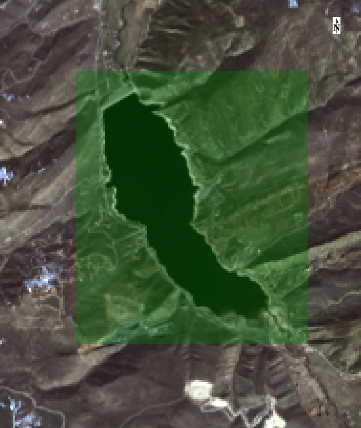
Figure 1: Original image with green ROI overlay

To start the process, I brought all of my data into IDL and got the reference to my current ENVI instance.

; Get the current envi instance

e = ENVI(/current)

 

; Get the data collection

DataColl = e.Data

 

; A Landsat 8 OLI dataset consists of one TIFF file per band,

; with an associated metadata file (*_MTL.txt). Open the

; metadata file to automatically read the gains and offsets.

 

IMG_File = File_Search('C:\MyData, '*_MTL.txt')

Raster = e.OpenRaster(IMG_File)

 

; A ENVI ROI that encapsulates the study area

ROI_File = File_Search('C:\MyData\ROIs', '*.xml')

oROI = e.OpenROI(ROI_File[0], PARENT_RASTER=Raster[0])

 

; Set the name for the output shapefile

output_SHP = 'C:\Output\Lake.shp'

Once I had the data in IDL, I subset the images to contain only my region of interest and convert the digital numbers to radians.

; Get the extent of the ROI

extent =  oROI.GetExtent(Raster[0])

 

; Subset the image to the extent of the study region

Subset = OBJARR(n_elements(Raster))

foreach Band, Raster, index do Subset[index] = Band.Subset(Sub_rect = extent)

 

; Get the radiometric calibration task from the catalog of ENVI tasks.

RadCal_Task = ENVITask('RadiometricCalibration')

 

; Define inputs. Since radiance is the default calibration method

; you do not need to specify it here.

RadCal_Task.Input_Raster = Subset[0] ; Bands 1-7

RadCal_Task.Output_Data_Type = 'Double'

 

; Define output raster URI

RadCal_Task.Output_Raster_URI = e.GetTemporaryFilename()

 

; Run the task

RadCal_Task.Execute

 

Now that the imagery is in a workable state, I calculated the normalized difference water index (NDWI) and thresholded the results to just pull out large bodies of water.

; Calculate a modification of normalized difference water index (NDWI)

 

; Xu, H. Modification of normalized difference water index (NDWI) to enhance  ; open water features in remotely sensed imagery. Int. J. Remote Sens. 2006,  ; 27, 3025–3033.

 

Green = RadCal_Task.Output_Raster.GetData(Bands=2)

SWIR = RadCal_Task.Output_Raster.GetData(Bands=5)

 

MNDWI = (Green - SWIR) / (Green + SWIR)

 

; Make a binary mask of just the water

Water = MNDWI gt .7 

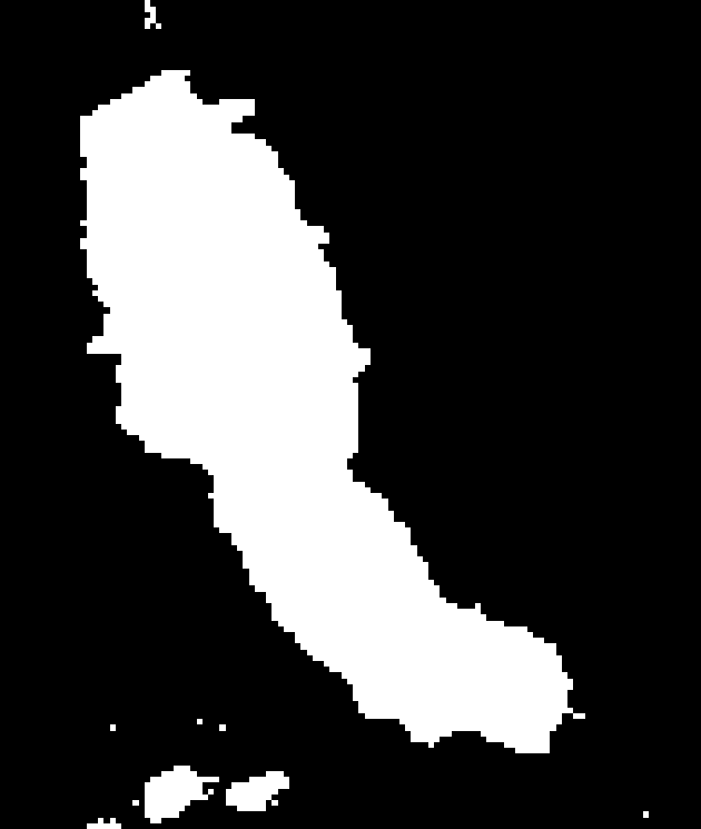
Figure 2: Binary mask of water regions

Since I was only interested in the large lake in the center of the image, I found which region had the most pixels and isolated that one.

; Find how many different regions there are in the image

Labeled_Water = LABEL_REGION(water,/ALL_NEIGHBORS)

 

; Find the number of pixels in each region (exclude zeros)

Region_Stats = lonarr(max(Labeled_Water))

foreach region, findgen(max(Labeled_Water)-1)+1, index do $

Region_Stats[index] = n_elements(where(Labeled_Water eq region))

 

; select the region with the most pixels

junk = max(Region_Stats,Region_pos)

 

; add zero position back in

Region_pos++

Through the use of contour, it was possible to find all of the pixels around the edge of the lake. This is very important for when we begin building our shapefile.

; Get the location of all the pixels around the edge of the target

Labeled_Water = Labeled_Water eq Region_pos

contour, Labeled_Water, PATH_INFO=path_info, path_xy=path_xy,$

  /PATH_DATA_COORDS, LEVELS=[1]

 

; Make sure that the first and last points match

if path_xy[0,-1] ne path_xy[0,0] and path_xy[1,-1] ne path_xy[1,0] then $

  path_xy = [[path_xy], [path_xy[*,0]]]

 

; convert from file location to map location

SpatialRef = RadCal_Task.Output_Raster.SpatialRef

SpatialRef.ConvertFileToMap, path_xy[0,*],path_xy[1,*], MapX, MapY

Now that all the shoreline pixels have been accounted for, it is possible to build the final output, the shapefile.

; create the shp file

oShp = obj_new('IDLffShape', output_SHP, /UPDATE, ENTITY_TYPE=5)

 

; Add the attributes

oShp->AddAttribute, 'Name', 7, 15

 

; create the new entity

ent = {IDL_SHAPE_ENTITY}

 

; set the entity index

entity_index = 0

 

; populate the entity

ent.SHAPE_TYPE = 5

ent.ISHAPE = entity_index

ent.N_VERTICES = n_elements(mapX)

ent.BOUNDS[0] = min(mapx)

ent.BOUNDS[1] = min(mapy)

ent.BOUNDS[2] = 0.0

ent.BOUNDS[3] = 0.0

ent.BOUNDS[4] = max(mapx)

ent.BOUNDS[5] = max(mapy)

ent.BOUNDS[6] = 0.0

ent.BOUNDS[7] = 0.0

ent.VERTICES = ptr_new([MapX,MapY])

 

; Populate the attribute

attr = oShp->GetAttributes(/ATTRIBUTE_STRUCTURE)

attr.ATTRIBUTE_0 = 'My Target'

 

; Add the entity to the shapefile

oShp->PutEntity, ent

 

; add the attribute to the shapefile

oShp->SetAttributes, entity_index, attr

 

; Close the shapefile

OBJ_DESTROY, oShp

 

; Create the projection file

prj_name = file_dirname(output_SHP) + path_sep() + file_basename(output_SHP, '.shp') + '.prj'

openw, lun, prj_name, /get_lun

writeu, lun, byte(Spatialref.COORD_SYS_STR)

close, lun

free_lun, lun

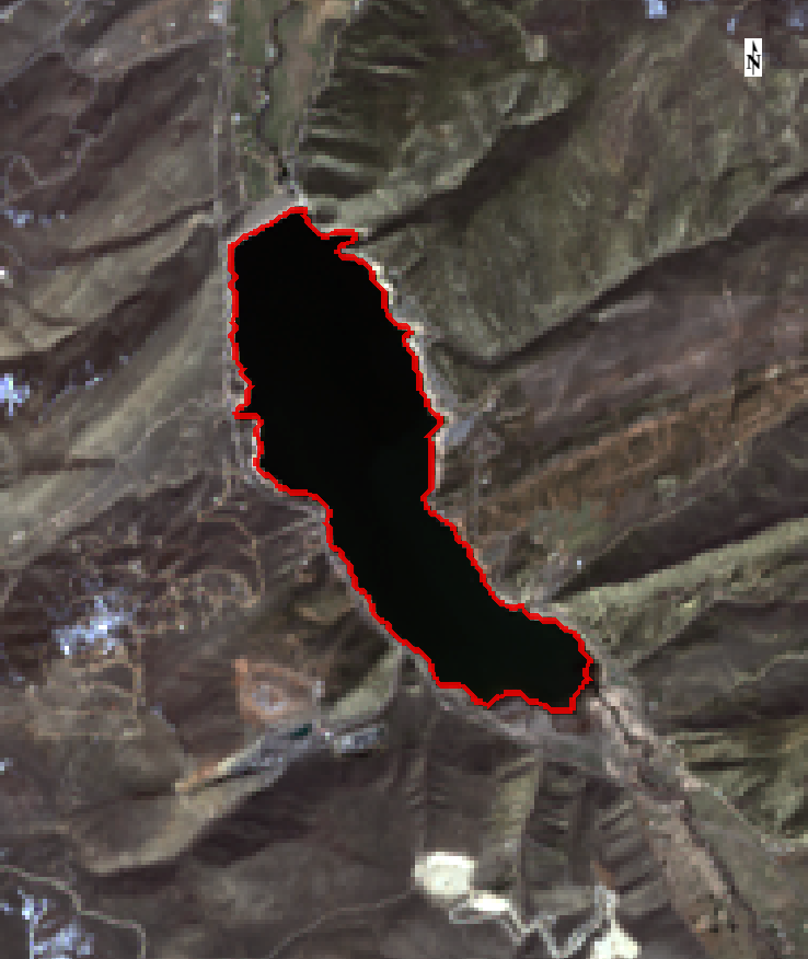
Figure 3: Image with final shapefile displayed in red

I hope this helps explain how to link a few different IDL and ENVI functions together in order to go from a raster to a vector.