Find the Finder
Anonym
Recently I was tasked with finding a QR code in an image and
then computing its location and. I learned that the first step in locating a QR
code is discerning the finder points. In QR codes there are three finder
points located at the furthest reaches of three of the corners. These finder
points are made up of white and black pixels and regardless of the rotation of
the code, a cross-section of one finder point will look like the following.
B W B B B W B
B = Black pixel; W =
White pixel
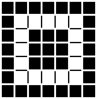
With this pattern of points being fixed and the ratio of
ring counts, with respect to the center block, being for the outer black ring,
  for the inner, white ring, I
found that it was possible to use the contour
procedure and a little math to pull out these finder points.
for the inner, white ring, I
found that it was possible to use the contour
procedure and a little math to pull out these finder points.

Figure 1: Input Image
To locate the finder points, I first opened the image and
stripped out a single band. Then I converted the image to a binary image and
coded any gaps that were formed by the conversion.
; open envi
e
= envi()
; open the image
oRaster = e.openRaster(inputfile)
; strip out single
band
band1 = oRaster.GetData(Bands=0)
; convert to binary
image
data = band1 gt 128
; close gaps
data =MORPH_Open(data,
REPLICATE(1,3,3))
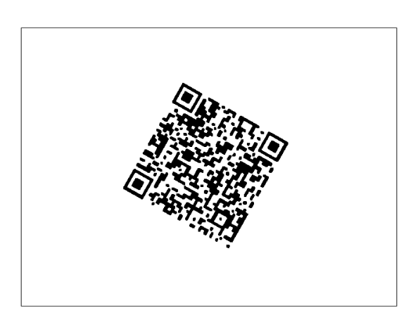
Figure 2: Binary image
Once I had a binary image, I computed the contour lines for
the full image. I then added each contour line to the previous contour line.
This step results in an image where contours that overlap have a much higher
value than those that do not.
; get the contours
of the image
contour, data,
PATH_INFO=path_info, path_xy=path_xy,$
/PATH_DATA_COORDS,
LEVELS=[0,1]
; build overlapping
image
overlap_img = bytarr(oRaster.ns,
oRaster.nl)
; create a
container for the ROIs, we will use them again
oROIs = make_array(n_elements(path_info), /OBJ)
for i = 0 , n_elements(path_info)-1 do begin
; get the end pos
end_pos =
(path_info[i].offset) + (path_info[i].n)-1
; get the points
pts =
path_xy[*,(path_info[i].offset):end_pos]
; last point has to
be the same as the first
xs = [[pts[0,*]],[pts[0,0]]]
ys = [[pts[1,*]],[pts[1,0]]]
; create the ROI
oROIs[i] = OBJ_NEW('IDLanROI', xs, ys)
; compute the mask
Mask =
oROIs[i]->ComputeMask(INITIALIZE=0, DIMENSIONS=[oRaster.ns,$
oRaster.nl],$
Mask_Rule=2)
; convert to binary
Mask = Mask eq 255
; add the mask to
the image
overlap_img =
overlap_img + Mask
endfor
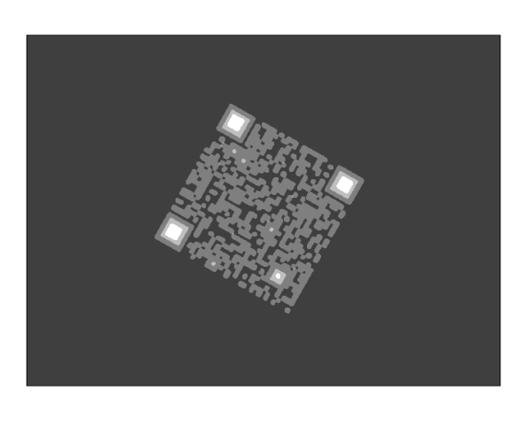
Figure 3: Overlapping contour image
Once the overlapping image was created, I searched for
regions that satisfy the and ring ratio rule. If any
contour groups were found, the center of mass of each grouping was recorded.
; get the max
number of overlaps in the image
max_overlap = max(overlap_img)
; set the desired
ratios
desired_ratio1 = 2. + (2./3.)
desired_ratio2 = 1. + (7./9.)
; create a
container for the finder points
finder_cm = []
for i = 0 , n_elements(path_info)-1 do begin
; compute the mask
Mask =
oROIs[i]->ComputeMask(INITIALIZE=0, DIMENSIONS=[oRaster.ns,$
oRaster.nl],$
Mask_Rule=2)
; convert to binary
Mask = Mask eq 255
;Mask overlap image
StudyArea =
overlap_img * Mask
;compute the
histogram of the image
Hist = HISTOGRAM(StudyArea,
LOCATIONS=pos, NBINS=nbins, BINSIZE = 1, MIN=1,$
MAX=max_overlap)
; if there are more
or less than 3 values, then discard it
pos = where(Hist ne 0)
if n_elements(pos) eq 3 then begin
; get the counts
for each bin
vals = float(hist[pos])
;calculate the
ratios
;outer black ring /
inner
ratio1 = vals[0] / vals[2]
;white ring / inner
ratio2 = vals[1] / vals[2]
; check that the
difference is desired ratio
ratio1_dif_percent = ratio1 / desired_ratio1
ratio1_dif_percent = abs(ratio1_dif_percent - 1.)
ratio2_dif_percent = ratio2 / desired_ratio2
ratio2_dif_percent = abs(ratio2_dif_percent - 1.)
; if they are
within 60%, save as a finder point
if ratio1_dif_percent lt .3 and ratio2_dif_percent lt .3 then begin
; calculate the
center of mass
StudyArea =
StudyArea gt 0
Mass = Total(StudyArea)
center_x = Total( Total(StudyArea, 2) * Indgen(oRaster.ns) )
/ Mass
center_y = Total( Total(StudyArea, 1) * Indgen(oRaster.nl) )
/ Mass
; record the center
finder_cm =
[[finder_cm],[center_x,center_y]]
endif
endif
endfor
Last, but not least, I took a moment to plot the results and
admire the fruits of my labor.
; display the input
image
im = image(oRaster.GetData(interleave='bsq') )
; plot the location
of the finder points on top of the input image
for i = 0 ,n_elements(finder_cm[0,*])-1 do $
p = SCATTERPLOT(finder_cm[0,i],finder_cm[1,i],$
OVERPLOT = im,
AXIS_STYLE=0, SYM_COLOR='red',$
SYM_FILL_COLOR='blue', SYM_FILLED=0, SYM_SIZE=2,$
SYMBOL='o',SYM_THICK=4)
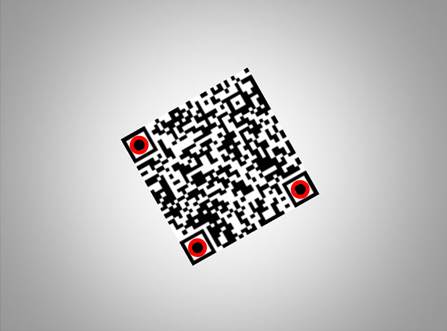
Figure 4: Final results
I hope that you got something out of this demo. If not how
to locate a finder point, then perhaps how to use contours in a new and
exciting way.