First Valley Shadow Detection
Anonym
Shadows can be difficult to deal with when introduced into an analysis pipeline. There are many different ways in which to deal with shadows, but I’ve found that one of the easiest ways is to simply mask them out. I work primarily with agricultural data and row-planted crops in particular. In this type of data, the shadows are cast on bare earth between rows, because of that they can be masked out without much heartache, assuming that your target material is the vegetation itself. Depending on what type of imagery is being used, shadows are normally one of the darkest, if not the darkest, surfaces in the image. This assumption can be used to our advantage—in a histogram of the imagery, the shadows should fall at the lower end.
For example, in this image of an orange orchard, the shadows are the darkest feature and thus fall at the bottom of the histogram.
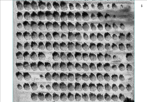
Figure 1: NIR image of orange orchard
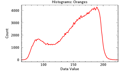
Figure 2: Histogram of figure 1
By looking at the imagery, you can see that there is a distinctive valley between two major features. Using the NIR First Valley Method (Jan-Chang, Yi-Ta, Chaur-Tzuhn, & Shou-Tsung, 2016), you can isolate the local minima then use that as the upper bound of a threshold used for shadow masking. The local minima can be easily derived by using the method presented in the support document entitled: Finding multiple local max/min values for 2D plots with IDL.
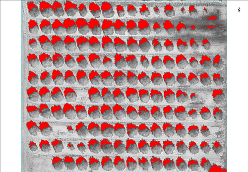
Figure 3: Shadows displayed in red
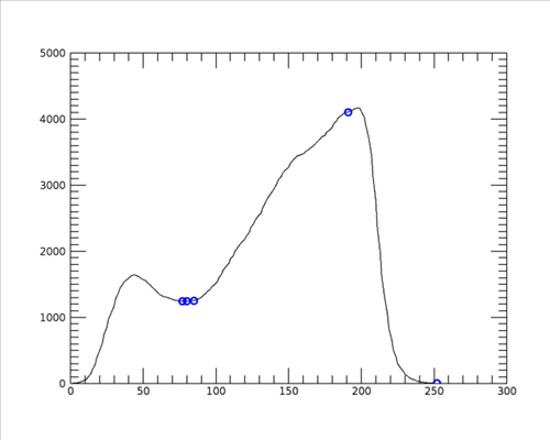
Figure 4: First valley identified
function local_max_finder, datax, datay, minima = minima compile_opt idl2 ;initialize list max_points = list() data_x = datax data_y = datay
;check for keyword, flip the sign of the y values if keyword_set(minima) then data_y = -datay ;iterate through elements for i=1, n_elements(data_y)-2 do begin
;previous point less than i-th point and next point less than i-th point if ( (data_y[i-1] le data_y[i]) AND (data_y[i] ge data_y[i+1])) then max_ points.add, i endfor ;return an array of the indices where the extrema occur return, max_points.toarray() end
pro ShadowFinder compile_opt IDL2 ; Select your image e = envi(/current) oRaster = e.UI.SelectInputData(/Raster, bands = bands) ; Check for single band if N_ELEMENTS(bands) gt 1 then begin MESSAGE, 'Input raster may only contain 1 band', /INFORMATIONAL return endif ; Pull the data out of the image data = oRaster.GetData(bands = bands, pixel_state = pixel_state) ; Convert data to float data = float(bytscl(data)) ; Mask all values in the image bkgrd_pos = where(pixel_state ne 0) data[bkgrd_pos] = !VALUES.F_NAN ; find all local minima based off the histogram of the image h = histogram(data, LOCATIONS=xbin) ; Remove zero values non_zeros = where(h ne 0) h = h[non_zeros] xbin = xbin[non_zeros] ; Get the number of points n_pts = n_elements(h) ; Smooth data (7 pixel moving average) boxcar = 7 p1 = (boxcar - 1) / 2 p2 = boxcar - p1 for i = 0 , n_pts-1 do begin pos = [i-p1:i+p1] pos = pos[where((pos ge 0) and (pos le n_pts-1))] h[i] = mean(h[pos]) endfor MINIMA = local_max_finder(xbin, h, /MINIMA) x_extrema = xbin[MINIMA] y_extrema = h[MINIMA] ; Plot all local minima p = plot(xbin, h) p3 = scatterplot(x_extrema, y_extrema, /current, /overplot, $ symbol = 'o', sym_color = 'b', sym_thick = 2) ; Create a shadow mask mask = bytarr(oRaster.ns, oRaster.nl) mask[where(data le x_extrema[0])] = 1 ; create a new metadata object metadata = ENVIRasterMetadata() metadata.AddItem, 'classes', 2 metadata.AddItem, 'class names', ['Background', 'Shadow'] metadata.AddItem, 'class lookup', [[0,0,0],[255,0,0]] metadata.AddItem, 'data ignore value', 0 metadata.AddItem, 'band names', 'Shadows' ; Create a classification image oClass = e.CreateRaster(e.GetTemporaryFileName(), mask, SPATIALREF = oRaster.SPATIALREF, $ data_type = 1, metadata = metadata) oClass.save ; Add the new class image to envi e.data.add, oClass end
References
Jan-Chang, C., Yi-Ta, H., Chaur-Tzuhn, C., & Shou-Tsung, W. (2016). Evaluation of Automatic Shadow Detection Approaches Using ADS-40 High Radiometric Resolution Aerial Images at High Mountainous Region. Journal of Remote Sensing & GIS.