Hyperspectral Data Reduction
The Spectral Hourglass Series: Part 3
Anonym
Before we begin we must reaffirm the end goal of this process: to find the most spectrally pure, or spectrally unique, pixels (endmembers) within the data set and to map their locations and sub-pixel abundances. Following the step of atmospheric correction we move on to Spectral Data Reduction. Determining the inherent dimensionality of a dataset will allow the analyst to ignore “noisy” data, and identify the number of spectrally distinguishable endmembers through the separation of information from noise.
A hyperspectral image contains a truly overwhelming amount of information, and the efficient and accurate identification of spectral bands containing the most information is a necessary first step. It will be later on that we can use our expertise and other ENVI® tools to identify the endmembers. What we accomplish in this step can be thought of as removing some of the clutter to see our data more clearly.
To accomplish this task of focusing solely on the pure endmembers found within our dataset, we perform a Minimum Noise Fraction (MNF) Transform. The MNF Transform alters the data to allow the analyst to subset a large number of the spectral bands due to the fact that the vast majority of unique spectral information will be contained within the first few MNF Transform bands (Boardman, J.W., 1993, “Automating Spectral Unmixing of AVIRIS DATA Using Geometry Concepts,” In Summaries of the Fourth Annual JPL Airborne Geoscience Workshop, JPL Publ. 93-26, Vol. 1, Jet Propulsion Laboratory, Pasadena, CA, pp. 11-14). In favor of describing how this is employed in ENVI, I will leave it up to our fine documentation center to deliver a much more detailed explanation of MNF Transform and its implementation within ENVI.
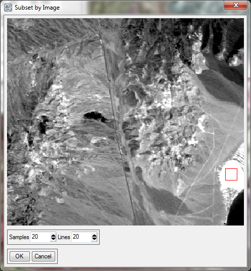
One can accomplish this task of spectral data reduction through the use of the ENVI interface. The first portion of this transform consists of estimating the noise statistics from the data using a shift difference technique. You can accomplish this in ENVI by selecting a spatial subset of spectrally uniform data to then calculate a noise statistic baseline. A homogenous group of pixels should demonstrate a similar spectral signature; variance within the spectra is assumed to be the result of noise and thus a noise statistic baseline can be calculated.
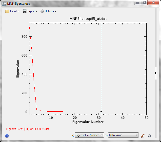
After some moments of processing ENVI will display the MNF transformed image as well as display a profile containing the MNF Eigenvalues. Bands with large eigenvalues (greater than 1) contain data, and bands with eigenvalues near or less than one contain noise. Recall the file we are using, cup95eff.int, which is a hyperspectral image that only contains fifty spectral bands. This is of importance because the number of spectral bands in your data will always be equal to the highest eigenvalue number.
The MNF Eigenvalues plot displayed shows that we will be able to subset a large number of spectral bands. After eigenvalue number 30 the eigenvalue falls below one, and we know that we can essentially discard nearly half of the data, even more if you what you seek in your imagery is relatively abundant within the scene. A quick note; many people will find a high eigenvalue number to be of importance so ENVI does not discard any of the information, it is up to the user to decide what is and is not important to their pursuit.
MNF Band 1 contains the largest eigenvalue and as a result the largest amount of variance. It is necessary to visually inspect the transform bands and the Band Animation Tool makes this task extremely easy. Within the Band Animation tool you will be able to cycle through all of the transform bands to determine which bands contain strictly noise and will not aide in the identification of endmembers. The first few bands will appear similar to grayscale images and as you get to MNF Band 15 and 20 you can seethe image more closely resembles a TV with bad signal.
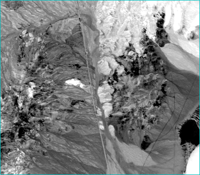
MNF Band 1
Through viewing the bands created by the MNF Transform tool we can start to weed out the superfluous data and focus only on the most interesting information.
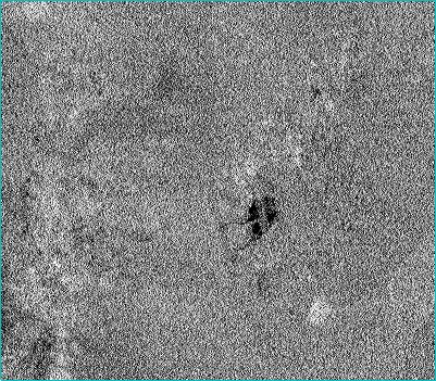
MNF Band 20
Although the vast majority of the pixels in MNF Band 20 seem to be very noisy, the dark region could highlight a homogenous grouping of pixels with unique spectra. Further investigation of the spectral profile of those pixels and comparison against a spectral library will allow us to identify the presence of Alunite, that is further along in the spectral hourglass workflow.
We are well on our way to extracting the most pure endmembers from our dataset with the help of some high-powered ENVI tools. The next few steps will begin to rely more heavily on the expertise of the user as well as the n-D Visualizer tool found within ENVI.
You can also go the programmatic route and write scripts to perform an MNF transform using the ENVIForwardMNFTransformTask and ENVIInverseMNFTransformTask routines.
Read The Spectral Hourglass Series: Part 4, Spatial Data Reduction and Pixel Purity Index
Read The Spectral Hourglass Series: Part 2, Spatial/Spectral Browsing and Endmembers