IDL's HISTOGRAM function

IDL's HISTOGRAM function

IDL's HISTOGRAM function is one of the most versatile functionsI can think of. It can be very fast and efficient for a number of common tasks.

1. Plotting a histogram is an effective way to investigate statisticalproperties of data. A probability density graph quickly shows the distribution:

IDL> a = randomn(seed, 100000)+15.5+3*randomn(seed, 100000)

IDL> p = plot(location,histogram(a,nbins=1000,location=location),'r')

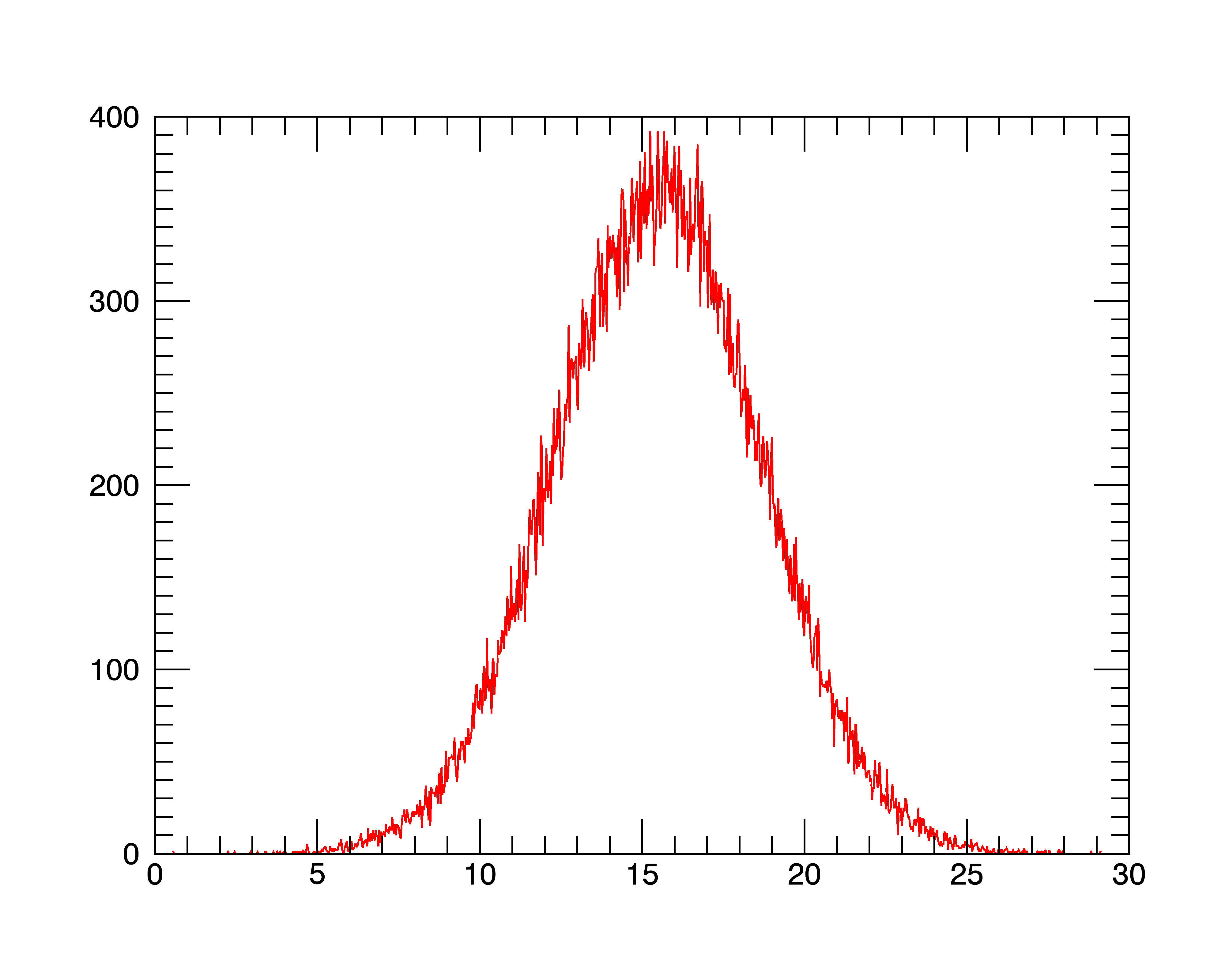
From the histogram, you could quickly conclude that asuitable range for BYTSCL might be MIN=10.0, MAX=20.0.

2. Finding percentiles in a programmatic way can be doneusing lookups in the cumulative histogram, for example if you want to find the5% and 95% in a dataset:

IDL> a = randomn(seed, 100000)+15.5+3*randomn(seed, 100000)

IDL> location[value_locate(total(histogram(a,nbins=1000,location=location),/cumulative)/a.length,[0.05,0.95])]

      10.285119       20.638901

Which shows that about 90% of the values are between 10.29and 20.64.

3. Finding the most common number in an array of integers.

IDL> arr = [3,7,34,5,8,8,5,31,5,8]

IDL> location[where(histogram(arr) eq max(histogram(arr,location=location)))]

       5       8

This shows a tie between 5 and 8 for the most abundant valuein the array.

4. Sorting can also be performed with HISTOGRAM. For example2-D sorting into a grid and computing the mean "F" value for eachgrid tile:

IDL> x = 45*randomu(seed, 100000)

IDL> y = 32*randomu(seed, 100000)

IDL> f = 5.5*randomn(seed, 100000) + 16

IDL> grid_index = floor(x + floor(y)*ceil(max(x)))

IDL> h = histogram(grid_index, min=0, binsize=1,reverse_indices=rev)

IDL> f_means = dblarr(ceil([max(x),max(y)]))

IDL> for i=0,h.length-1 do if h[i] gt 0 then f_means[i] = mean(f[rev[rev[i]:rev[i+1]-1]])

Check one of the values using the slower "WHERE"approach:

IDL> f_means[6,8]

      15.784905433654785

IDL> mean(f[where(floor(x) eq 6 and floor(y) eq 8)])

       15.784905