Quickly Read and Display Data From a New File Format - Paleontology with IDL

Over time, you may run across data sets that you'd like to read in IDL, file formats that lack any built-in utilities in the language.

Quite frequently I use the following technique for building custom data readers for IDL in my work for the Custom Solutions Group.

A recent article I ran across described a newly-minted repository of paleontological data, including 3D models of bones of long-lost species. MorphoSource.org, is a Duke University project funded in part by grants from the National Science Foundation. Commercial use of the provided media is strictly prohibited, according to their website.

My goal was to see how easy it would be to read some of this data and display it in an interactive IDL display. It was very simple, indeed!

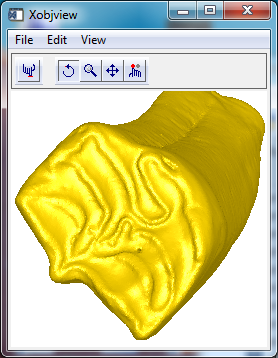
Searching the database I found a number of interesting data types, including 3D models. One example, shown above and copyright the Florida Museum of Natural History, is the tooth of a Calippus elachistus, an early horse-like mammal that may have roamed the area in Florida during the Miocene epoch.

I requested a user account from MorphoSource.org and their robot sent me back the OK to grab some data, for instructional and non-commercial use only, of course.

Drilling down a little further I located some ASCII-format "Avizo PLY"-format files. I've not worked with this type of file before, and IDL doesn't have a built-in reader, but opening the file in a standard text editor shows that the format is straightforward.

Given this information, it's easy to build a utility in IDL that will both read the data and display the 3D object.

Though we won't attempt to parse all the data in the file, we can quickly locate the two major pieces of data we need for visualization, the list of vertex coordinates and the connectivity of those vertices.

The header begins with the following

ply
format ascii 1.0
obj_info Format: Avizo PLY
element vertex 249741
property float32 x
property float32 y
property float32 z
element face 495182
property list uint8 int32 vertex_indices

What this tells me is that somewhere in the file there are 249741 vertices with floating point (X,Y,Z) coordinates and 495182 "faces" or connectivity lists. A connectivity list tells us how the indices in the vertex list connect to one another.

(In other files in the MorphoSource data sets, you may also find data for vertex coloring, which adds greater interest!)

There are some additional lines in the header which we will ignore.  The header ends with an "end_header" line.

The lines immediately after the header are series of three floating point elements, for example

end_header
34.6223 25.3743 11.5595
34.5367 25.4449 11.5501
34.6183 25.4799 11.5998

Gosh, those look like vertex coordinates, don't they?  Now we can follow a hunch that if we look down the file another 249741 lines (the vertex count), we'll find data in a different format.  Sure enough, we find a transition.

23.9367 23.4851 43.5914
24.1271 23.4578 43.5783
24.0427 23.5348 43.5879
3 0 4 1 0
3 1 2 0 0
3 3 8 7 0
3 8 3 0 0

The connectivity list of each line starts with the number of vertices in a polygon's face.In this case they're all triangles, therefore the value is "3". Following the vertex count are the three zero-based indices of the vertices that make up each triangular facet.The last number in each line may indicate whether the polygon is open or closed. They all have a value of 0, so we'll just ignore the fifth value.

Not coincidentally, these vertex and connectivity lists are precisely in the format that IDL's IDLgrPolygon object uses.

After downloading the file to my desktop, I'll read the contents of the file into a string array variable named "val".

file = 'UF-53577_M5794-5222_Calippus_elachistus.ply'
n = file_lines(file)
val = strarr(n)
openr, lun, file, /get_lun
readf, lun, val
free_lun, lun

Locate the line that starts with the text "element vertex". We'll split that line on spaces and pull out the third element.  That's the vertex count.

vertexline = where(val.startswith('element vertex'))
vertexcount = long((val[vertexline[0]].split(' '))[2]) 

Repeat for the polygon connectivity count, which starts with "element face".

polygonline = where(val.startswith('element face'))
polygoncount = long((val[polygonline[0]].split(' '))[2])

Create IDL arrays in which to store the vertices and polygons.

vertices = fltarr(3, vertexcount)
poly = lonarr(4, polygoncount)

Remove the header from the string array so we're positioned at the first line of vertices.

last = (where(val.startswith('end_header')))[0]
val = val[last + 1: *]

Loop over the lines containing the vertex data, and extract the values into the vertices array.

for i = 0L,  vertexcount - 1 do $
  vertices[0, i] = float(((val[i]).trim()).split(' '))

Remove the vertices from the start of the string array and repeat the procedure for the connectivity.

val = val[vertexcount:*]
for i = 0L, polygoncount - 1 do $
  poly[0, i] = (long(((val[i]).trim()).split(' ')))[0:3]

For the display, we only need two lines of code.  Populate an IDLgrPolygon object with our data.

opolygon = idlgrpolygon(vertices, poly = poly, style = 2, color = !color.gold)

Finally, display the data in one of IDL's interactive tools, XOBJVIEW.

xobjview, opolygon

Did this horse have a cavity, or is the hole in the crown a spot that's been drilled for sampling?

Below is an example routine that incorporates the code shown above, and generates an MP4 animation in your temporary directory.  You will need to request a MorphoSource account to download your own PLY-format file as input. Feel free to generalize the code for a more robust PLY-format solution.

pro read_ply, dir, vertices
file = filepath('UF-53577_M5794-5222_Calippus_elachistus.ply')
n = file_lines(file)
val = strarr(n)
openr, lun, file, /get_lun
readf, lun, val
free_lun, lun
vertexline = where(val.startswith('element vertex'))
vertexcount = long((val[vertexline[0]].split(' '))[2])
polygonline = where(val.startswith('element face'))
polygoncount = long((val[polygonline[0]].split(' '))[2])
vertices = fltarr(3, vertexcount)
poly = lonarr(4, polygoncount)
last = (where(val.startswith('end_header')))[0]
val = val[last + 1: *]
for i = 0L,  vertexcount - 1 do $
vertices[0, i] = float(((val[i]).trim()).split(' '))
val = val[vertexcount:*]
for i = 0L, polygoncount - 1 do $
poly[0, i] = (long(((val[i]).trim()).split(' ')))[0:3]
;poly = reform(poly, poly.length, /overwrite)
om = idlgrmodel()
opolygon = idlgrpolygon(vertices, style = 2, poly = poly, color = !color.gold)
om->add, opolygon
mx = mean(vertices[0, *])
my = mean(vertices[1, *])
mz = mean(vertices[2, *])
om->translate, -mx, -my, -mz
xobjview, om, tlb = tlb, xsize = 256, ysize = 256
frames = list()
temppng = filepath(/tmp, 'frame.png')
for i = 0, 360, 3 do begin ; rotate
om->rotate, [1, 1, 0], 3
xobjview, refresh = tlb
xobjview_write_image, temppng, 'png'
frames.add, read_png(temppng)
file_delete, temppng
endfor
for i = 1, 100, 3 do begin ; zoom in
om->scale, 1.03, 1.03, 1.03
xobjview, refresh = tlb
xobjview_write_image, temppng, 'png'
frames.add, read_png(temppng)
file_delete, temppng
endfor
for i = 1, 100, 3 do begin ; zoom out
om->scale, 1/1.03, 1/1.03, 1/1.03
xobjview, refresh = tlb
xobjview_write_image, temppng, 'png'
frames.add, read_png(temppng)
file_delete, temppng
endfor
tempvid = filepath(/tmp, 'horsetooth.mp4')
ovid = IDLffVideoWrite(tempvid)
fs = (frames[0]).dim
vidstream = ovid.AddVideoStream(fs[1], fs[2], 24)
foreach frame, frames do $
t = ovid.put(vidstream, frame)
obj_destroy, ovid
spawn, tempvid
end