ENVI Orthorectification Module

ENVI Orthorectification Module Whitepaper

Introduction

Scientists, geospatial analysts, and technicians increasingly need to combine data from many sources in order to produce useful geospatial products for their customers. With the rise of commonly available high spatial resolution satellite imagery (such as QuickBird, GeoEye-1, and others), it’s more important than ever before to have accurate geospatial registration to ensure accurate data combination, overlay, and product fusion.

Geospatial registration accuracy needs for this kind of work can commonly exceed those provided by more commonly used approaches, such as RPC orthorectification and simple geometric registration. In these cases, only a true rigorous sensor model orthorectification will suffice. A effective solution has to work on many different operating systems, perform block bundle adjustments with multiple simultaneous sensor models, ground control points (GCPs) and tie points – all of which is provided in the ENVI Orthorectification Module.

NV5 Geospatial has partnered with Spacemetric, an image management solutions provider, who are experts in rigorous photogrammetric methods and orthorectification. The ENVI Orthorectification Module uses Spacemetric’s advanced models to quickly achieve high quality results.

Spacemetric’s solutions are based on rigorous photogrammetric methods. An explicit mathematical formulation defines the image capture process by describing the relationship between individual pixels as imaged by the sensor’s detector array and their location on the Earth. A sensor model characterizing the specific geometrical properties of an instrument provides an interface to the full range of photogrammetric functionality.

Orthorectification

Many factors contribute to the geometric properties of a remotely sensed image. The introduction of geometric distortions during image capture is inevitable and contributes to geospatial positioning errors, object artifacts and scale inconsistencies in geographically referenced imagery. The image acquisition geometry, the topographic relief of the image area, the optical fidelity of the sensor and the positional stability of the sensor each play a role in the amount and type of errors that are introduced.

Orthorectification is a process that removes the geometric distortions introduced during image capture and produces an image product that has planimetric geometry, like a map. Orthorectified imagery, also known as orthoimagery, is precisely registered to a ground coordinate system and the image scale is constant throughout the entire image. Orthorectified imagery is also free of artifacts, such as leaning objects and crooked linear features, due to relief displacement. These properties make orthoimagery ‘map accurate’ and the clear choice for applications that require accurate positional information and precise measurement of features.

Uses for Orthoimagery

Orthoimagery is an essential element to many geospatial information applications. It is most commonly used as an image base or contextual backdrop for a map to form a more complete visualization of the environment being represented. The photographic nature of orthoimagery is easily interpretable by users and often provides the most up-to-date information of the geography under study. Used with GIS data layers, orthoimagery can form rich geospatial data visualizations for cadastral mapping, urban planning, civil engineering, topographic mapping, site evaluations, transportation analysis and natural resource management.

Since orthoimagery is considered map accurate, it provides the ideal data source for digitizing planimetric map features like roads, utility assets, urban infrastructure and natural features. These feature classes can be collected off of the orthoimagery using manual ‘heads-up’ onscreen digitization or through more automated methods like object based feature extraction (e.g., ENVI Fx).

In a similar fashion, orthoimagery is useful for vector data verification tasks. Through the comparison of vector data against up-to-date orthoimagery, it is easy to identify feature omissions, misaligned features or otherwise out-of-date features in a geodatabase. For example, orthoimagery would clearly show when a road intersection is realigned to improve a safety condition.

Orthoimagery is also needed for precise three dimensional point coordinate determination, to accurately measure distances between two points and along routes, and to make unbiased areal calculations. These capabilities are important to engineering and military applications where mission success depends on information with the highest spatial accuracy.

Industry Segments Requiring Orthorectification:

• Civil Engineering
• Defense (Targeting, Engineering, Site Analysis)
• Economic Development
• Environmental Monitoring
• Forestry
• Natural Resource Management
• Real Property Inventory and Assessment
• Urban Planning
• Watershed Analysis

Approaches to Orthorectification

There are two common but different technical approaches to orthorectification. Each attempts to improve the accuracy of the absolute image pixel location through a reconstruction of the imaging geometry using elevation inputs. However, the methods differ in the number of input parameters used, the complexity of the sensor models employed and the exactness of the solution.

Orthorectification from Substitute Sensor Models (RPC or RSM)

The Rational Polynomial Coefficients (RPCs) and Replacement Sensor Model (RSM) methods describe a mathematical model that relates image space coordinates (sample and line position) to latitude, longitude and surface elevation. RPCs and RSMs are often referred to as “substitute sensor models” by photogrammetrists because they only approximate the exact physical model of the sensor. The substitute approach protects proprietary sensor designs and promotes system interoperability, since disparate sensor types are all handled the same way.

RPCs and RSM are computed via a photogrammetry technique that uses a collinearity equation to construct the sensor geometry, where the object point, perspective center, and image point are all on the same space line. The technique involves a series of nonlinear transformations that moves between image and ground coordinate systems. As such, these substitute sensor models are pseudo-projections and imagery using RPC or RSM should not be considered projected. Related imagery is generally still in its original acquisition state (straight off the sensor), but the ground coordinates for each image pixel are known and can be reported to the user. This means that the RPC solution is solved each time the ground coordinate for the pixel is requested.

ENVI supports RPC as a georeferencing schema for imagery and is also capable of performing RPC based orthorectification. Both capabilities are provided as part of the core ENVI product.

ENVI provides three levels of RPC orthorectification. The basic level is to orthorectify using RPCs and a static elevation value. More accuracy is obtained by orthorectifying with RPCs and a Digital Elevation Model (DEM). The most accuracy is gained by orthorectifying using RPCs, a DEM and Ground Control Points (GCPs). The RPC method of orthorectification tends to have a high bias error (absolute positioning error) and a much lower random error (internal variance or relative error); therefore, selecting even a single GCP can provide significant improvement in overall rectification accuracy.

Rigorous Orthorectification

Rigorous orthorectification is the most accurate method of image geolocation and geometric correction. Using the rigorous method, high accuracy image geolocation is accomplished by using photogrammetric methods that employ physical sensor models and advanced statistical treatment of elevation and geometric reference data. Systemic geometric errors in the imagery are corrected by applying formulas derived from first principles physics based models. The number of algorithms and formulas used in the rigorous method can number in the 100s and more.

In traditional orthorectification processes, random errors are typically accounted for through the use of well-distributed ground control points (GCPs). The use of GCPs in geometric correction involves collecting coordinates of known features on the ground that can be accurately located in the image. GCPs can either be collected from a Global Positioning System (GPS) in the field or measured from an existing map, and are defined in either a geographic (latitude and longitude) coordinate system or in a projected coordinate system, such as Universal Transverse Mercator (UTM). In addition to the use of GCPs, traditional orthorectification processes also use digital elevation models (DEMs) to correct for relief displacement. Sensor attitude and orientation are generally corrected by taking into account both exterior and interior orientation parameters of the sensor or camera.

The many advantages of the rigorous photogrammetric approach include:

• Highest possible geometrical accuracy for given input data
• Lower operational costs - method is highly stable and requires less external data such as ground control points
• Support of true image orthorectification with sub-pixel geolocation accuracy
• Full photogrammetric functionality readily available for any satellite or airborne sensor, with modest efforts required to develop a sensor model

Analytical Models

The rigorous method combines several analytical sub-models to construct a line-of- sight model (LOS) that describes how a pixel in a satellite image is projected onto the ground. Each of the sub-models can be independently modified or adjusted to improve the overall accuracy of the solution. It is important to note that each of these models is time dependent, meaning that the models are parameterized to accept inputs that change over the duration of the image collect. This is particularly important for imagery collected through scanning systems and collections from platforms that are relatively unstable in their flight or orbital trajectories. As a whole, the sub-models described below form a complete optical sensor model.

• Sensor model: The sensor model takes a pixel in the image and computes its look vector, or line-of-sight, in the sensor coordinate system. It also computes the time for the instance of this look. The sensor model is initialized with parameters specific for the sensor design. It can be a generic model for a push broom scanner, which will have parameters such as focal length, detector positions in the focal plane and scan-line time interval. Alternatively, it can be a highly specialized model for a more complicated sensor. The sensor model is the sub-model that is most often modified when implementing a new imaging system.

• Body model: The body model is used to rotate the look vector from the sensor coordinate system to the satellite body coordinate system. It is used to model either the intended off-nadir sensor mounts or the small misalignments in the nominal mount.

• Attitude model: The attitude model is used to rotate the look vector from the body coordinate system to the flight coordinate system. The rotations between these systems are due to deviations in platform attitude. This is a time-dependent variation, usually measured by devices such as earth horizon detectors, inertial measurement units, gyroscopes or star trackers. The attitude model is initiated by a set of time-coded attitude and/or attitude rate measurements. The time of the look is used to calculate the transformation to be used.

• Flight model: The flight model is used to rotate the look vector from the flight coordinate system to the Earth Centered Inertial (ECI) coordinate system. It is also used to calculate the position of the satellite. It employs orbital mechanics and is initiated by sets of parameters such as one or several ephemeris, several time-tagged position vectors or two-line elements. The time of the look is used to calculate the transformation and position to be used.

• Astronomical model: The astronomical model is used to transform the position and look vectors from the ECI system to the Earth Centered Rotating (ECR) coordinate system. It is primarily a rotation of the x-axis from the Vernal Equinox to the Greenwich Meridian. The transformation is time-dependent and the time of the look is used to calculate the transformation to be used.

• Intersection model: The intersection model calculates the intersection point between the look vector and an ellipsoidal Earth centered in the ECR system. The ellipsoidal height is also input to get a unique position. An atmospheric model is applied to correct for the deviation caused by atmospheric refraction.

• Geodesy model: The geodesy model transforms the Earth intersection point, expressed in ECR coordinates, to a geographic coordinate (longitude, latitude, orthometric height). It uses a geoid model to account for the irregularities in the Earth zero potential surface. The result is a coordinate in the WGS84 system.

• Map projection: The map projection transforms the geographic coordinate to a cartographic coordinate (x, y, h) by the use of a map projection that is suitable for the geographical area of the image. There are thousands of different map projec tions in use for different cartographic purposes all over the globe.

Block Bundle Adjustment

Prior to applying orthorectification to the imagery, the parameters of the line-of-sight model can be adjusted to fit a set of ground control points (GCPs). The block bundle adjustment, also known as Model Parameter Adjustment, is used to improve the geometrical accuracy in the output product. A GCP consists of a 3-dimensional ground coordinate (x, y, h) and its estimated accuracy (sx, sy, sh). An image point (IP) consists of a position in the satellite image (column, row) and its estimated accuracy (scolumn, srow). Marking the position of a GCP in the satellite image consequently gives a constraint on the model parameters. A number of such measurements give rise to a system of constraint equations that can be solved by least-squares adjustment.

Tie points (TPs) are image measurements that connect the same locations in different, but overlapping, images. In the model parameter adjustment, they are treated as IPs with small (zero) variance measured for GCPs with high (infinite) variance. This way, TPs, can conveniently be accommodated in the same generalized least-squares solution.

The goal of the least-squares adjustment is to minimize the error terms on all of the GCPs and tie points simultaneously. The optimal least-squares solution employs the “generalized least-squares” approach. This makes full use of all a priori information, including start values for the parameters and their estimated accuracies.

Applying Rigorous Orthorectification

Once the line-of-sight geometric model is established for an image, it can be used in image orthorectification. The steps involved are:

• Set the output frame parameters. This includes the choice of coordinate system (map projection), bounding rectangle and pixel size for the rectified image. A minimum frame that completely contains the rectified image can be calculated automatically.
• Associate a DEM with image to be orthorectified. If a DEM is not available, a static elevation can be substituted and used as a reference surface.
• Compute the locations of the output pixels in the input image. This inverse line-of- sight transform is not performed for every pixel as computationally this would be too costly. Instead, it is performed through the use of a regular grid over the image. The density of the grid is adjusted to be tight enough that a bilinear interpolation of positions within a grid cell is sufficiently accurate.
• Resample the input image by interpolating the non-integer positions of the output pixels. The interpolation method is selectable from among standard methods such as cubic convolution, bilinear and nearest neighbor.
• Save the rectified image to the specified image format.

ENVI Orthorectification Module

Geometric accuracy performance

Spacemetric software has achieved unsurpassed geometric accuracy in operational environments for many years. The models typically achieve ½ pixel accuracy or better with ground control of sufficient quality. This level of accuracy has been verified during many years of operational use and is documented in numerous technical papers, a selection of which are referenced below and are available for download through Spacemetric’s website (www.spacemetric.com).

Features

Easy-to-use Workflow Wizard

The ENVI Orthorectification module presents an easy-to-use interface and wizard- based workflow that steps the user through orthorectification setup, visualization of the results and final processing. The wizard dialogs have two control buttons at the bottom, which allow the user to maneuver backward and forward through the wizard. At any point throughout the orthorectification workflow, the project can be saved and later restored.

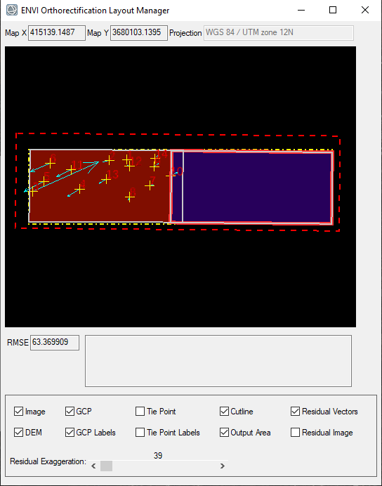
ENVI Orthorectification Layout Manager

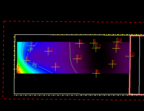
The Layout Manager provides a visual and tabular view of the current state of the orthorectification project. This feature enables the user to quickly assess the spatial coverage of all of the input data used to create an orthorectified product including images, DEMs, ground control points (GCPs), tie points, cutlines, and the output area. The dialog also shows tables of GCP and tie point locations, residual error vectors for each GCP, and the overall root mean square (RMS) error (Figure 1). Additionally, residual errors can be viewed as a residual error map (Figure 2).

The Layout Manager includes the following components setup in a tab interface format:

• Status Bar - indicates the cursor position in X and Y map units, according to the projection type listed in the Projection field.
• Draw Area - shows the spatial coverage (in map space) of the input images, DEMs, GCPs, tie points, cutlines, output area, and residuals.
• GCP Tab - contains a table that lists each selected GCP as shown in the Draw Area. The table lists the error magnitude for each point (under the Mag field). The following columns are provided for each GCP: ID, MapX, MapY, Elev, Image ID, Sample, Line, resX, resY, and Mag.
• Tie Point Tab - contains a table that lists each selected tie point as shown in the draw area. Each tie point is assigned an ID number. Columns list the image names, sample, line, and Map X/Y coordinates for each of the two images.
• Images Tab - lists the full paths to image files that will be used in processing.
• DEMs Tab - lists the full paths to DEM files that that will be used in processing.

As GCPs and tie points are added or removed to the project, the Layout Manager automatically updates to show the changes. The orthorectification model is recomputed any time GCPs or tie points are edited. It is easy to determine if the selected GCPs have broad spatial coverage across the input images and if there are enough tie points to cover image overlap regions. It is possible to view all of these components at the same time, or only show specific items of interest.

Broad Sensor Support

The ENVI Orthorectification Module supports a wide range of satellite and aerial based sensors. The module works with image data and accompanying metadata in native formats as delivered from the commercial data provider. For a full list of supported data formats, please see Appendix 1.

Custom sensor definitions can also be added for non-supported frame cameras by creating an exterior/interior orientation description in the form of an XML file. Contact Technical Support for more information.

Integration with Esri ArcGIS Workflows

Since the module is implemented in the ENVI processing environment, it is easy to take advantage of ENVI’s existing integration features with Esri ArcGIS tools and data formats. This adds orthorectification capability to existing ENVI image processing and Esri ArcGIS geoprocessing workflows.

Workflow

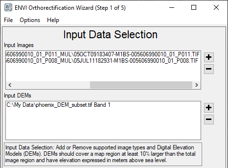
Step 1 – Select input imagery and DEM

The first step in the ENVI orthorectification workflow is to load the imagery and digital elevation models that will be used for processing (Figure 3). The files are chosen from the current set in the Available Bands List. This is also the step where the user can load a previous saved orthorectification project.

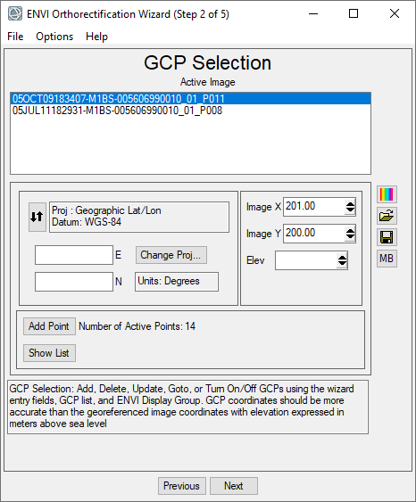
Step 2 - Collecting and Editing Ground Control Points

After the input data has been selected, the wizard proceeds to the GCP selection panel (Figure 4). In this step, image pixels are associated with points on the ground whose locations are known through a horizontal coordinate system and vertical datum. These points are called ground control points (GCPs). The controls in this step of the wizard allow the user to optionally restore GCP files, to add new GCPs, and to edit existing GCPs.

Once at least four GCPs have been added to the project, the Layout Manager will display information on the root mean square error (RMSE) of the model solution given the input GCPs. For the best orthorectification results, the user should try to minimize the overall root mean square error by refining the positions or removing the GCPs with the largest associated errors.

The RMSE error information is presented in tabular form, through a residual vector map and in a residual surface image map. These displays make it easy to see which GCPs are contributing the most error in the solution.

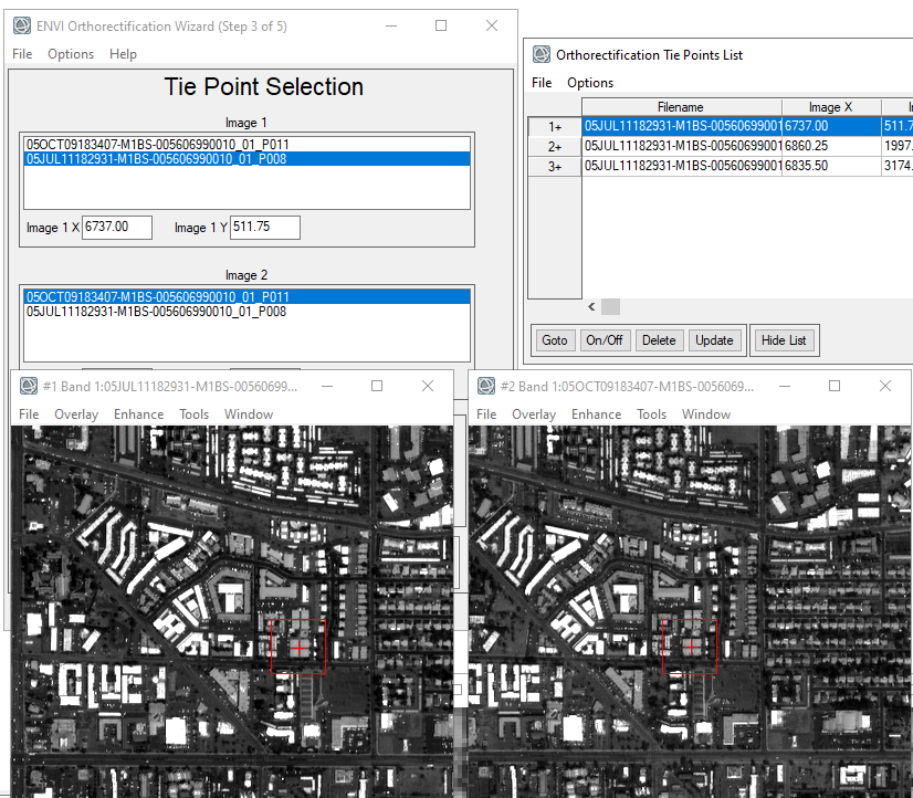
Step 3 - Collecting and Editing Tie Points

If more than one image is being orthorectified, the user may choose to establish tie points (TPs) between the images. Tie points are pairs of pixels located in overlapping images that represent the same object or feature location on the earth. Along with GCPs, tie points are an integral part of the bundle adjustment and account for most of the relative accuracy in the orthorectified product.

In this step, the user can define the tie points for image-to-image registration between two image display groups (Figure 5). The controls in this step of the wizard also allow the user to restore previously created tie point files, add new tie points, and to edit existing tie points. Tie point collection is an optional step. The orthorectified solution can be computed without tie points.

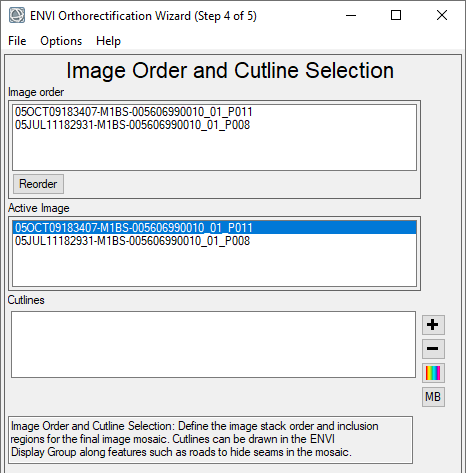
Step 4 - Reordering Images and Defining Cutlines

The fourth step in the workflow defines the image extent of the orthorectified product and specifies which areas between two or more overlapping images should appear in the final output. With each input image, the user must: define the hierarchy of the image relative to the others, and define an optional cutline for the image (Figure 6).

An image order list is used to define how multiple images are ordered in the final output. This list is populated with the image filenames added to the workflow in step number one. The image at the top of the list will be ordered first, followed by the second image, and so forth. Image ordering only pertains to areas of overlap between two or more images.

Cutlines are polygons that are used in combination with image ordering to define areas to keep in the final output. A cutline is an inclusion polygon, similar to a cookie cutter, applied to one or more images. Cutlines are defined by drawing a polygon on the image in an ENVI display group.

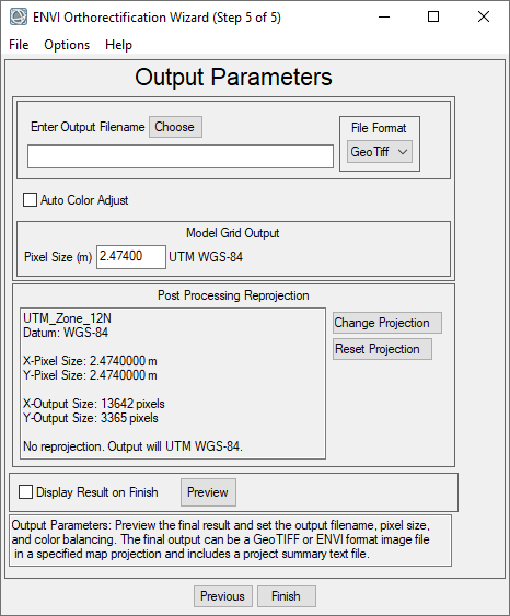
Step 5 - Selecting Output Parameters

In the final step of the workflow, the user specifies the output map projection, pixel size, filename and path (Figure 7). For projects that include multiple images, an auto color-adjust routine is available to balance tonal differences between the scene content in the output mosaic. Spacemetric developed the underlying method, which uses a least-squares adjustment to ensure radiometric consistency among the scenes that comprise the mosaic.

When the “Finish” button is clicked, ENVI builds the full-resolution orthorectified output and displays the processing status. Once processing is complete, the orthoimagery is added to the Available Bands List.

Value and Benefits

Fast and Accurate

The ENVI Orthorectification Module was developed in partnership with world-class orthorectification experts, Spacemetric. By fully integrating the Spacemetric solution with ENVI, users can achieve accurate orthorectification results within a familiar ENVI environment.

Easy to Use

Existing orthorectification packages are extremely difficult to use for non-photo- grammetrists. The ENVI Orthorectification Module is easy to use, as it has a wizard interface to guide the user through the necessary steps. Visualization uses standard ENVI displays, and controls for tasks such as selecting ground control points or tie points use existing ENVI tools.

Convenient

The ENVI Orthorectification Module will allow scientists and technicians alike to achieve best-possible registration results with the data available to them. The module allows users to use a minimum of an input image and DEM, will accept multiple images (from multiple sensors), multiple DEMs, ground control points (GCPs), or tie points, in any combination. In addition, because it is a fully integrated add-on module for ENVI, users can perform all orthorectification tasks in a single, familiar product and have access to ArcGIS through ENVI’s integration and partnership with Esri.

Availability

The ENVI Orthorectification Module is available with the release of ENVI 4.6.1.