Not All Supernovae Are Created Equal: Rethinking the Universe’s Measuring Tools

6/3/2025

Rethinking the Reliability of Type 1a Supernovae How do astronomers measure the universe? It all starts with distance. From gauging the size of a galaxy to calculating how fast the universe is expanding, measuring cosmic distances is essential to understanding everything in the sky. For nearby stars, astronomers use... Read More >

Using LLMs To Research Remote Sensing Software: Helpful, but Incomplete

5/26/2025

Whether you’re new to remote sensing or a seasoned expert, there is no doubt that large language models (LLMs) like OpenAI’s ChatGPT or Google’s Gemini can be incredibly useful in many aspects of research. From exploring the electromagnetic spectrum to creating object detection models using the latest deep learning... Read More >

From Image to Insight: How GEOINT Automation Is Changing the Speed of Decision-Making

4/28/2025

When every second counts, the ability to process geospatial data rapidly and accurately isn’t just helpful, it’s critical. Geospatial Intelligence (GEOINT) has always played a pivotal role in defense, security, and disaster response. But in high-tempo operations, traditional workflows are no longer fast enough. Analysts are... Read More >

Thermal Infrared Echoes: Illuminating the Last Gasp of a Dying Star

4/24/2025

This blog was written by Eli Dwek, Emeritus, NASA Goddard Space Flight Center, Greenbelt, MD and Research Fellow, Center for Astrophysics, Harvard & Smithsonian, Cambridge, MA. It is the fifth blog in a series showcasing our IDL® Fellows program which supports passionate retired IDL users who may need support to continue their work... Read More >

A New Era of Hyperspectral Imaging with ENVI® and Wyvern’s Open Data Program

2/25/2025

This blog was written in collaboration with Adam O’Connor from Wyvern. As hyperspectral imaging (HSI) continues to grow in importance, access to high-quality satellite data is key to unlocking new insights in environmental monitoring, agriculture, forestry, mining, security, energy infrastructure management, and more.... Read More >

1 2 3 4 5 6 7 8 9 10 Next Last

«

June 2025

»

Sun

Mon

Tue

Wed

Thu

Fri

Sat

25

26

27

28

29

30

31

1

2

3

4

5

6

7

8

9

10

11

12

13

14

15

16

17

18

19

20

21

22

23

24

25

26

27

28

29

30

1

2

3

4

5

7346 Rate this article:

4.1

Creating GOES-16 ABI Aerosol Detection Visualizations of the Marshall Fire

David Starbuck Monday, May 2, 2022

The fall of 2021 was extremely dry in Colorado, and on December 30th when category 2 hurricane force winds hit the area, an urban wildfire erupted that led to the largest loss of property in Colorado history. The Marshall Fire destroyed over one thousand structures in the cities of Superior and Louisville, and in unincorporated Boulder County. Residents in the area often had only minutes to evacuate, many fleeing with only the clothes on their backs.

Along with the 1,000 plus structures that were lost, many other homes and businesses experienced severe smoke damage. While the extreme winds and prolonged drought made the conditions ideal for uncontrollable fire behavior, residents are now facing the realization that this situation might not have been a rare instance of a perfect storm. In the aftermath of the Marshall Fire, the Colorado Front Range, with a large population near a fire climax ecosystem, is coming to terms with the real possibility of endemic wildfires and a fire season that is now year-round.

Using Imagery to Study Wildfires

Geospatial imagery can be used to study pre-fire conditions, monitor conditions during a fire and evaluate damage after. Data from the Advanced Baseline Imager (ABI), a sensor on the L3Harris built GOES-16 platform, allows us to study all types of weather phenomena at high temporal, spatial and spectral resolution. Certain bands highlight smoke, others different sized aerosols, and others fire itself. The more people who can access, analyze and visualize ABI data, the more we can learn from these types of events and how they impact people’s lives, health, air travel safety, etc.

ABI datasets have a direct read out link to NOAA and facilities like those at the University of Wisconsin and other sites for operational use in forecasting but are also publicly available via AWS S3 buckets. This blog post provides code examples and demonstrates how anyone can use the IDL® programming language to pull GOES-16 ABI data from AWS S3 for this date, create RGB images that show smoke dynamics and extents, and create an Aerosol Detection data product.

Step-by-Step Guide To Access ABI Data

The first step to access ABI data is pulling the data from AWS S3 using the IDLnetURL object in IDL. I used the AWS Amazon S3 API guide to figure out how to fill out the IDLnetURL parameters – Amazon S3 - Amazon Simple Storage Service. Using this guide, I wrote the following routine to query the Goes-16 S3 data.


	function dj_goes_16_s3_query, prefix=prefix, print=print
  compile_opt idl2

  s3UrlObject = obj_new('idlneturl')
  bucket = 'noaa-goes16'
  region = 'us-east-1'
  s3UrlObject.setProperty, url_host = bucket + '.s3.' + region + '.amazonaws.com'
  
  urlQuery = 'list-type=2&delimiter=/'
  
  if keyword_set(prefix) then begin
    urlQuery = urlQuery + '&prefix='+prefix
  endif 
  
  
  
  keyList=list()
  dateList = list()
  sizeList = list()
  
  gotAll = 0 
  startAfter = ''
  initUrlQuery = urlQuery 
  while (gotAll eq 0) do begin
    urlQuery = initUrlQuery
    if startAfter ne '' then begin
      urlQuery = urlQuery + '&start-after=' + startAfter
      startAfter = ''
    endif
    
    s3urlObject.setproperty, url_query= urlQuery
    result = s3urlObject.get()

    parsedData = xml_parse(result)
    
    if ((parsedData['ListBucketResult']).haskey('Contents')) then begin
      contents = ((parsedData['ListBucketResult'])['Contents'])
      for  awsKeyIndex=0L, n_elements(contents)-1 do begin
        keyList.add, (contents[awsKeyIndex])['Key']
        dateList.add, (contents[awsKeyIndex])['LastModified']
        sizeList.add, (contents[awsKeyIndex])['Size']
      endfor
      if keyword_set(print) then begin
        outArray = strarr(3,n_elements(keyList))
        outArray[0,*] = transpose(keyList.toArray())
        outArray[1,*] = transpose(dateList.toArray())
        outArray[2,*] = transpose(sizeList.toArray())
        print, '---------------------------------'
        print, 'Key, Date, Size
        print, '---------------------------------'
        print, outArray
      endif
    endif

    prefixList= list()
    if ((parsedData['ListBucketResult']).haskey('CommonPrefixes')) then begin
      commonPrefixes = ((parsedData['ListBucketResult'])['CommonPrefixes'])
      if n_elements(commonPrefixes) eq 1 then begin
        prefixList.add, commonPrefixes['Prefix']
      endif else begin
        for prefixKeyIndex=0L, n_elements(commonPrefixes)-1 do begin
          prefixList.add, (commonPrefixes[prefixKeyIndex])['Prefix']
        endfor
      endelse
      if keyword_set(print) then begin
        print, '---------------------------------'
        print, 'Prefixes'
        print, '---------------------------------'
        print, transpose(prefixList.toArray());objListStructor['prefixlist']
      endif
    endif
    
    if ((parsedData['ListBucketResult'])['IsTruncated'] eq 'true') then begin
      startAfter = keyList[-1]
    endif else begin
      gotAll = 1
    endelse
 
  endwhile

  returnHash = hash()
  returnhash['keylist'] = keyList
  returnhash['datelist'] = dateList
  returnhash['sizelist'] = sizeList
  returnhash['prefixlist'] = prefixList  
  
  obj_destroy, s3UrlObject

  return, returnhash
end

In this routine, I used “noaa-goes16” as the bucket and “us-east-1” as the region.


		 s3UrlObject = obj_new('idlneturl')
  bucket = 'noaa-goes16'
  region = 'us-east-1'
  s3UrlObject.setProperty, url_host = bucket + '.s3.' + region + '.amazonaws.com'

I used “list-type=2” with the “delimiter=/” as parameters to the “url_query” property. Running the query returns a list of the keys (files) and prefixes (subdirectories) available in the top level of the bucket. Without the delimiter, the response that all the files in the bucket creates a very long list.


		  s3urlObject.setproperty, url_query='list-type=2&delimiter=/'
  result = s3urlObject.get()

The response will be an XML object which can be parsed using the xml_parse routine. After that the keys and prefixes can be extracted.


	parsedData = xml_parse(result)

Running “dj_goes_16_s3_query” without any prefix specified, will produce the following result:


		IDL> topLevelQuery = dj_goes_16_s3_query(/print)
---------------------------------
Key, Date, Size
---------------------------------
Beginners_Guide_to_GOES-R_Series_Data.pdf 2021-04-02T17:12:02.000Z 5887019
Version1.1_Beginners_Guide_to_GOES-R_Series_Data.pdf 2021-03-23T15:49:55.000Z 3578396
index.html 2021-09-27T19:48:14.000Z 32357
---------------------------------
Prefixes
---------------------------------
ABI-L1b-RadC/
ABI-L1b-RadF/
ABI-L1b-RadM/
ABI-L2-ACHAC/
ABI-L2-ACHAF/
ABI-L2-ACHAM/
ABI-L2-ACHTF/
ABI-L2-ACHTM/
ABI-L2-ACMC/
ABI-L2-ACMF/
ABI-L2-ACMM/
…
SUVI-L1b-Fe284/

I then used the “prefix” parameter to query the keys and prefixes under a specific prefix. For example, I used the following call to view the prefixes available under “ABI-L1b-RadC/”:

IDL> productTypeLevelQuery = dj_goes_16_s3_query(/print, prefix='ABI-L1b-RadC/')
---------------------------------
Prefixes
---------------------------------
ABI-L1b-RadC/2000/
ABI-L1b-RadC/2017/
ABI-L1b-RadC/2018/
ABI-L1b-RadC/2019/
ABI-L1b-RadC/2020/
ABI-L1b-RadC/2021/
ABI-L1b-RadC/2022/

I continued this process with further subdirectories and found the following structure for each key:

<Product Type>/<year>/<day>/<hour>/<filename.nc>

I used the GOES-16: True Color Recipe — Unidata Python Gallery tutorial as a guide on how to generate RGB images from the GOES-16 data. According to this tutorial, the Level 2 Multichannel formatted data product should be used (ABI-L3-MCIMP). Therefore, I used the following query to determine which files are available for that type for the data 12/30/2022:

IDL> hourlevelQuery = dj_goes_16_s3_query(/print, prefix='ABI-L2-MCMIPC/2021/364/17/')

I printed the result and found that the first key available was:

ABI-L2-MCMIPC/2021/364/17/OR_ABI-L2-MCMIPC-M6_G16_s20213641701172_e20213641703545_c20213641704048.nc

I wrote the following routine to download files from the bucket.

function dj_goes_16_s3_download, key, outputdirectory=outputdirectory
  compile_opt idl2
  
  s3UrlObject = obj_new('idlneturl')
  bucket = 'noaa-goes16'
  region = 'us-east-1'
  s3UrlObject.setProperty, url_host = bucket + '.s3.' + region + '.amazonaws.com'
  
  fileBaseSplitString = strsplit(key, '/', /EXTRACT)
  fileBaseName = fileBaseSplitString[-1]
  s3urlObject.setProperty, url_path=Key

  if (keyword_set(outputdirectory)) then begin
    outputFilename = filepath(filebasename, ROOT_DIR=outputDirectory)
  endif else begin
    outputFilename = fileBaseName
  endelse
  
  ;if file already exist, don't re-download it
  if (file_test(outputFilename)) then begin
    objectFile = outputfilename
  endif else begin
    objectFile = s3urlObject.get(filename=outputFileName)
  endelse

  return, objectFile
end

To download a file, I ran “dj_goes_16_s3_download” using “ABI-L2-MCMIPC/2021/364/17/OR_ABI-L2-MCMIPC-M6_G16_s20213641701172_e20213641703545_c20213641704048.nc” as the key:

IDL>objectFile = dj_goes_16_s3_download('ABI-L2-MCMIPC/2021/364/17/OR_ABI-L2-MCMIPC-M6_G16_s20213641701172_e20213641703545_c20213641704048.nc')

The GOES-16 data are NetCDF and can be parsed using the ncdf_parse.

data = ncdf_parse(objectFile, /read_data) 

center_lon = data['geospatial_lat_lon_extent', $
        'geospatial_lon_nadir', '_DATA']
xscale = data['x', 'scale_factor', '_DATA']
xoffset = data['x', 'add_offset', '_DATA']
x_radians = data['x', '_DATA']*DOUBLE(xscale) + xoffset
yscale = data['y', 'scale_factor', '_DATA']
yoffset = data['y', 'add_offset', '_DATA']
y_radians = data['y', '_DATA']*DOUBLE(yscale) + yoffset

I used the following commands to get the red, blue and true green values from the data. I set the maximum value to 2,000 when scaling it because I looked at the histograms and found that most of the data resided below that value.

redBand = bytscl(data['CMI_C02', '_DATA'], max=2000)
greenBand = bytscl(data['CMI_C03', '_DATA'], max=2000)
blueBand = bytscl(data['CMI_C01', '_DATA'], max=2000)

trueGreen = bytscl(0.45*redBand + 0.1*greenBand + 0.45*blueBand)

bandDims = size(redBand, /DIMENSIONS)
rgbArray = fltarr(3,bandDims[0],bandDims[1])
rgbArray[0,*,*] = redBand
rgbArray[1,*,*] = trueGreen
rgbArray[2,*,*] = blueBand

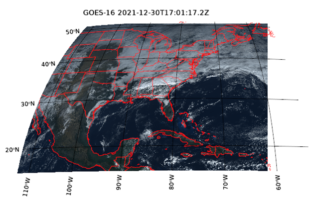
I then used the image function to display the data:

windowDimX = 800
windowDimY = 450
margin = [.2,.2,.1,.1]
i = IMAGE(bytscl(rgbArray), x_radians, y_radians, $
 MAP_PROJECTION='GOES-R', $
 margin=margin,    $
 GRID_UNITS='meters', $
 CENTER_LONGITUDE=center_lon, $
 DIMENSIONS=[windowDimX,windowDimY], $
 TITLE='GOES-16 '+ data['time_coverage_start', '_DATA'])
mg = i.MapGrid
mg.label_position = 0
mg.clip = 0 
mc = MAPCONTINENTS(/COUNTRIES, COLOR='red')
mc = MAPCONTINENTS(/US, COLOR='red')

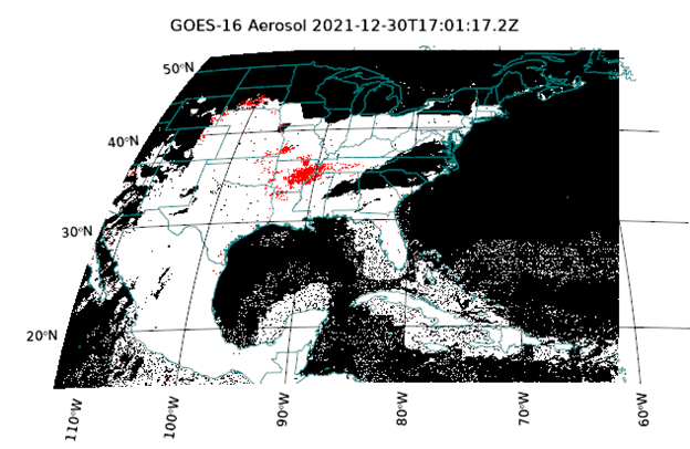
I then followed a similar procedure to display the aerosol detection. The aerosol data is a byte array with three values (0, 1, 255). I added a colortable to set 0 to black, 1 to red and 255 to white.

objectFile = dj_goes_16_s3_download('ABI-L2-ADPC/2021/364/17/OR_ABI-L2-ADPC-M6_G16_s20213641701172_e20213641703545_c20213641705442.nc')
data = ncdf_parse(objectFile, /read_data)
center_lon = data['geospatial_lat_lon_extent', $
   'geospatial_lon_nadir', '_DATA']
xscale = data['x', 'scale_factor', '_DATA']
xoffset = data['x', 'add_offset', '_DATA']
x_radians = data['x', '_DATA']*DOUBLE(xscale) + xoffset
yscale = data['y', 'scale_factor', '_DATA']
yoffset = data['y', 'add_offset', '_DATA']
y_radians = data['y', '_DATA']*DOUBLE(yscale) + yoffset
aerosol = data['Aerosol', '_DATA']
rgbTable = bytarr(3,255)
rgbTable[*,0] = 255
rgbTable[0,1] = 255
rgbTable[1,1] = 0
rgbTable[2,1] = 0
windowDimX = 800
windowDimY = 450
margin = [.2,.2,.1,.1]
i = IMAGE(aerosol, x_radians, y_radians, $
  MAP_PROJECTION='GOES-R', GRID_UNITS='meters', $
  margin=margin, $
  CENTER_LONGITUDE=center_lon, $
  RGB_TABLE=rgbTable, $
  DIMENSIONS=[windowDimX,windowDimY], $
  TITLE='GOES-16 Aerosol '+ data['time_coverage_start', '_DATA'])

The following program is an example program that uses “dj_goes_16_s3_query” and “dj_goes_16_s3_download” to generate an animation of true color images using the GOES-16 data around the Marshall Fire from 17:00-22:00 UTC. If you run this program with the aerosol keyword, it will generate an animation using the Aerosol Detection Goes-16 data product.

	
	pro dj_example_plot_areosol_goes_aws, aerosol=aerosol

  compile_opt idl2

  windowDimX = 800
  windowDimY = 450
  margin = [.2,.2,.1,.1]
  
  topLevelQuery = dj_goes_16_s3_query(/print)
  prefixes = (topLevelQuery['prefixlist']).toArray()
  multiChannelIndex = where(strmatch(prefixes,'*ABI-L2-MCMIPC*'))
  aerosolIndex = where(strmatch(prefixes, '*ABI-L2-ADPC*'))
  if keyword_set(aerosol) then begin
    productTypeLevelQuery = dj_goes_16_s3_query(prefix=prefixes[aerosolIndex[0]], /print)
  endif else begin
    productTypeLevelQuery = dj_goes_16_s3_query(prefix=prefixes[multiChannelIndex[0]], /print)
  endelse
  
  prefixes = (productTypeLevelQuery['prefixlist']).toArray()
  yearIndex = where(strmatch(prefixes,'*2021*'))
  yearLevelQuery = dj_goes_16_s3_query(prefix=prefixes[yearIndex[0]], /print)
  
  prefixes = (yearLevelQuery['prefixlist']).toArray()
  dayIndex = where(strmatch(prefixes,'*364*'))
  dayLevelQuery = dj_goes_16_s3_query(prefix=prefixes[dayIndex[0]], /print)
  
  hoursPrefixes = dayLevelQuery['prefixlist']

  ;Create video object for projected video
  if keyword_set(aerosol) then begin
    oVid = IDLffVideoWrite('aerosol_projected_output.mp4',FORMAT='mp4')
    vidstream = oVid.AddVideoStream(windowdimx,windowdimy,10)
  endif else begin
    oVid = IDLffVideoWrite('projected_output.mp4',FORMAT='mp4')
    vidstream = oVid.AddVideoStream(windowdimx,windowdimy,10)
  endelse


  ;Store a list of the hours prefixes for
  ;hoursPrefixes = objListStructor['prefixlist']

  for hoursIndex = 17L, 21 do begin

    hourLevelQuery = dj_goes_16_s3_query(prefix=hoursPrefixes[hoursIndex], /print)
    objectKey = (hourLevelQuery['keylist'])
    
    for objectKeyIndex = 0L, n_elements(objectKey)-1 do begin
      
      objectFile = dj_goes_16_s3_download(objectKey[objectKeyIndex])

      data = ncdf_parse(objectFile, /read_data)

      print, 'Time start = ', data['time_coverage_start', '_DATA']

      ; Extract the center longitude and radiance data
      center_lon = data['geospatial_lat_lon_extent', $
        'geospatial_lon_nadir', '_DATA']
      ; radiance = data['Rad','_DATA']

      ; Compute the X/Y pixel locations in radians
      xscale = data['x', 'scale_factor', '_DATA']
      xoffset = data['x', 'add_offset', '_DATA']
      x_radians = data['x', '_DATA']*DOUBLE(xscale) + xoffset
      yscale = data['y', 'scale_factor', '_DATA']
      yoffset = data['y', 'add_offset', '_DATA']
      y_radians = data['y', '_DATA']*DOUBLE(yscale) + yoffset

      if (keyword_set(aerosol)) then begin
        aerosol = data['Aerosol', '_DATA']
        smoke = data['Smoke', '_DATA']

        rgbTable = bytarr(3,255)
        rgbTable[*,0] = 255
        rgbTable[0,1] = 255
        rgbTable[1,1] = 0
        rgbTable[2,1] = 0

        if (obj_valid(i)) then begin
          i.setdata, aerosol, x_radians, y_radians
          i.title = 'GOES-16 Aerosol '+ data['time_coverage_start', '_DATA']
        endif else begin
          ; Use the GOES-R (GOES-16) map projection
          i = IMAGE(aerosol, x_radians, y_radians, $
            MAP_PROJECTION='GOES-R', GRID_UNITS='meters', $
            margin=margin, $
            CENTER_LONGITUDE=center_lon, $
            RGB_TABLE=rgbTable, $
            DIMENSIONS=[windowDimX,windowDimY], $
            TITLE='GOES-16 Aerosol '+ data['time_coverage_start', '_DATA'])

          i.limit = [38,-106, 41, -101]
          mg = i.MapGrid
          mg.label_position = 0
          mg.clip = 0
          mg.linestyle = 'none'
          mg.box_axes = 1

          mc = MAPCONTINENTS(/COUNTRIES, COLOR='teal')
          mc = MAPCONTINENTS(/US, COLOR='teal')
          
          annotationArrow = arrow([-105,-105.1],[40.5,40.05], /DATA,$
            COLOR='blue', $
            /CURRENT)

          t2 = text(-104.995, 40.51,'Approx. Smoke Origin', color='blue', /DATA, font_style=1)
        endelse

        time = ovid.put(vidStream, i.copywindow())
        print, time

      endif else begin
        redBand = bytscl(data['CMI_C02', '_DATA'], max=2000)
        greenBand = bytscl(data['CMI_C03', '_DATA'], max=2000)
        blueBand = bytscl(data['CMI_C01', '_DATA'], max=2000)

        trueGreen = bytscl(0.45*redBand + 0.1*greenBand + 0.45*blueBand)

        bandDims = size(redBand, /DIMENSIONS)
        rgbArray = fltarr(3,bandDims[0],bandDims[1])
        rgbArray[0,*,*] = redBand
        rgbArray[1,*,*] = trueGreen
        rgbArray[2,*,*] = blueBand
        
        ;Apply squareroot stetch to improve image clarity. 
        rgbArray = sqrt(rgbArray/255)*255

        ; Use the GOES-R (GOES-16) map projection
        if obj_valid(i) then begin
          ;skip frame at 2021-12-30T19:31:17.2Z
          if (data['time_coverage_start', '_DATA'] ne '2021-12-30T19:31:17.2Z') then begin
            i.setData, rgbArray, x_radians, y_radians
            i.title = 'GOES-16 '+ data['time_coverage_start', '_DATA']
          endif         
        endif else begin
          i = IMAGE(bytscl(rgbArray), x_radians, y_radians, $
            MAP_PROJECTION='GOES-R', $
            margin=margin, $
            GRID_UNITS='meters', $
            CENTER_LONGITUDE=center_lon, $
            DIMENSIONS=[windowDimX,windowDimY], $
            TITLE='GOES-16 '+ data['time_coverage_start', '_DATA'])

          i.limit = [38,-106, 41, -101]
          mg = i.MapGrid
          mg.label_position = 0
          mg.clip = 0
          mg.linestyle = 'none'
          mg.box_axes = 1

          mc = MAPCONTINENTS(/COUNTRIES, COLOR='red')
          mc = MAPCONTINENTS(/US, COLOR='red')
          
          annotationArrow = arrow([-105,-105.1],[40.5,40.05], /DATA,$
             COLOR='red', $
             /CURRENT)
             
          t2 = text(-104.995, 40.51,'Approx. Smoke Origin', color='red', /DATA, font_style=1)
        endelse
        ;skip frame at 2021-12-30T19:31:17.2Z
        if (data['time_coverage_start', '_DATA'] ne '2021-12-30T19:31:17.2Z') then begin
          time = ovid.put(vidStream, i.copywindow())
          print, time
        endif
      endelse
    endfor
  endfor
  ovid = 0
end

Thanks for following along. And, be on the lookout for some additional blogs accessing and creating visualizations with GOES, EUMETSAT and other instruments. IDL provides flexible access to complex data and code and it can be shared with colleagues via the IDL Virtual Machine – a free way to run IDL Code! My team specializes in solving tough problems with imagery using ENVI® and IDL and bridging other programming languages. If you have a project we might be able to help with, shoot me an email at GeospatialInfo@NV5.com.