An N-body College Reunion
A little over 30 years ago, the professor in my sophomore quantum mechanics class gave us a free range assignment. We could use a computer to solve any sort of physics problem. It need not be related to quantum in any way, which was just as well since I've never grokked the wave function in fullness.
This was back in the day when students training for careers in basic sciences were expected to know how to write their own analysis applications, and not mindlessly press buttons on spreadsheets or web pages. In no small part because the latter hadn't been invented yet.
I chose a problem in astrophysics. At the time there was academic research being performed on simplified galactic collisions, and the plots in the scientific journals were fascinating to me. N-body problems were well beyond my grasp, unless N was one or two.
I had no access to supercomputers, and my classical mechanics training was only at the freshman level.
But I liked pretty pictures.
It was challenging at the time to debug Fortran PLOT10 programs when one needed to plan for additional wait time in line at the campus computing center for the output and it took an hour for a Calcomp plotter to produce the (garbage) graph the (garbage) code was generating.
Unfortunately, my attempt burned down, fell over, and sank into the swamp. I vaguely recall I received an orange slice and a participant’s ribbon for the effort. Thanks for not failing me, Prof. Dutta.
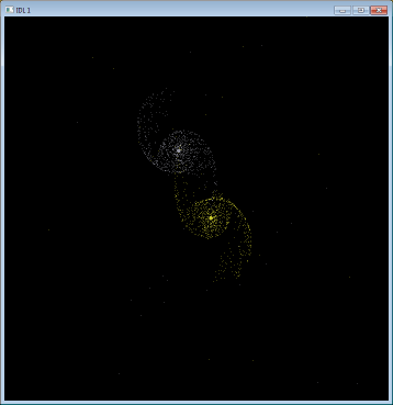
But a decade later, and with access to IDL, I reattempted the feat during a competition to produce demos for IDL 5.0.
The results were more satisfying visually, if not more realistic physically.
I've left the code below more or less intact. It’s a main application. Dig the DEVICE, DECOMPOSED=0 and parentheses instead of square brackets – 100% OG, and I don’t mean Object Graphics.
Essentially, two point masses represent galactic centers and 1000 mass-less test points (“stars”) are given initial circular paths around those centers. Both galactic centers then move relative to their center of mass with some initial conditions intended to provoke a visually appealing, if physically bogus, result.
I wrote a number of variants on this theme, color-coded the stars by speed relative to the center of mass, added other “galactic” masses, etc. If you find this interesting, try varying initial parameters such as the relative masses and velocities.
; initialization section
G = 4.4999e-12 ; pc^3 y^-2 Msol^-1
epsilon = 1.e5 ; yr
snapshot = 16.e6 ;yr
nsnapshots = 16
maxradius = 15d3 ; pc
initialsep = 2.*maxradius
Ngalaxies = 2
GalaxyColors = [150, 200]
Nsuns = 1000
vx = dblarr(Ngalaxies*(Nsuns + 1)) & vy = vx & vz = vx & x = vx & y = vx
z = vx & m = vx & rdist=  vx & thetadist = vx & ax = vx & ay = vx & az = vx
m(0) = 10.d9 ; Msol
x(0) = initialsep/2.*cos(!pi/4.)
y(0) = initialsep/2.*sin(!pi/4.)
m(1) = 9.d9 ;Msol
x(1) = -x(0)
y(1) = -y(0)
speed = 2*sqrt(G*m(1)/initialsep)
vx(0) = -speed*sin(!pi/4.)/2.
vy(0) = speed*cos(!pi/4.)/2.
vx(1) = -vx(0)*sqrt(m(0)/m(1))/3.
vy(1) = -vy(0)*sqrt(m(0)/m(1))/3.
; execution section
device, decomposed = 0
iseed = 138987
for i = Ngalaxies, Ngalaxies*(Nsuns + 1) - 1 do begin
rdist(i) = randomu(iseed) * maxradius
thetadist(i) = randomu(iseed)*2*!pi
m(i) = 1.
endfor
for j = 0, ngalaxies - 1 do begin
for i = ngalaxies + j*nsuns, ngalaxies + (j + 1)*nsuns - 1 do begin
x(i) = rdist(i)*cos(thetadist(i)) + x(j)
y(i) = rdist(i)*sin(thetadist(i)) + y(j)
z(i) = 0.
speed = sqrt(G*m(j)/max([Abs(rdist(i)),1.e-30]))
vx(i) = -speed*sin(thetadist(i)) + vx(j)
vy(i) = speed*cos(thetadist(i)) + vy(j)
vz(i) = 0.
endfor
endfor
loadct,15
!ignore = -1
!x.style = 2
!y.style = 2
window, 1, xsize=700, ysize=700, xpos = 0, ypos = 0
wset, 1
for t = -epsilon, snapshot*(nsnapshots - 1), epsilon do begin
ax(*) = 0 & ay = ax & az = ax
for j = 0, NGalaxies - 1 do begin
r = sqrt((x - x(j))^2 + (y - y(j))^2 + (z - z(j))^2)
r3 = r^3 > 1.e-20
Gprod = -G*m(j)/r3
ax = Gprod*(x-x(j)) + ax
ay = Gprod*(y-y(j)) + ay
az = Gprod*(z-z(j)) + az
endfor
vx = vx + epsilon*ax
vy = vy + epsilon*ay
vz = vz + epsilon*az
x = x + epsilon*vx
y = y + epsilon*vy
z = z + epsilon*vz
if (t eq -epsilon) then begin
rs = 1.5*initialsep
plot, [rs, -rs], [rs, -rs], color = 0
closedcircles,sym=1
for i = 0, NGalaxies - 1 Do Begin
oplot,[x(i),x(i)],[y(i),y(i)],color=galaxycolors(i)
endfor
!psym = 3
for i = 0, NGalaxies - 1 Do Begin
indices = indgen(nsuns) + (i*nsuns) + Ngalaxies
oplot, x(indices), y(indices), color=galaxycolors(i)
endfor
oldx = x
oldy = y
endif else begin
;
;	Erase the previous frame
;
closedcircles,sym=1
oplot,oldx(0:NGalaxies-1),oldy(0:NGalaxies-1), color = 0
!psym = 3
oplot, oldx, oldy, color = 0
;
;	Draw the galaxy centers
;
closedcircles,sym=1
for i = 0, NGalaxies - 1 Do Begin
oplot,[x(i),x(i)],[y(i),y(i)],color=galaxycolors(i)
endfor
;
;	Draw the stars
;
!psym = 3
for i = 0, NGalaxies - 1 Do Begin
indices = indgen(nsuns) + (i*nsuns) + Ngalaxies
oplot, x(indices), y(indices), color=galaxycolors(i)
endfor
;
;	Save the coordinates
;
oldx = x
oldy = y
empty
endelse
endfor
end
You will also need the following support routine.
Pro ClosedCircles, Symbol_Radius = Symbol_Radius, Color = Color
On_Error, 2
Ang = (360./47.*Findgen(48))/!RaDeg
X = Cos(Ang)
Y = Sin(Ang)
If (N_Elements(Symbol_Radius) ne 0) then Begin
	X = X * Symbol_Radius
	Y = Y * Symbol_Radius
EndIf
If (N_Elements(Color) eq 0) then Begin
	UserSym, X, Y, /Fill
EndIf Else Begin
	UserSym, X, Y, /Fill, Color = Color
EndElse
!P.PSym = 8
Return
End