Bridge to Bridge (R to Python to IDL)

Within ENVI and IDL there are many different classification schemes and functions that can be used to aid in analyzing your data (ENVI classification documentation). However, on occasion you may notice that we have not had a chance to code in your favorite ones yet or perhaps the method you wish to use is so cutting edge that it is a little ahead of our development cycle. If that is the case then there is a chance that the method you desire may be found within the ever-expanding R statistical package.  As you may have read last week on the IDL Data Point blog we are now able to call R though the use of the IDL to Python Bridge! This week, I wanted to show you another example of how this can be done and some of the tricks to get you going.

If you have not followed the steps on setting up your IDL, Python, and R environments yet, it may be a good idea to do that now. Once you are all up and running we can get into the meat of this post. The purpose of this post is not to go into extensive detail on all of the nuances of these bridges but rather show a fun example of how to visualize a classification tree and point out a few pitfalls along the way.

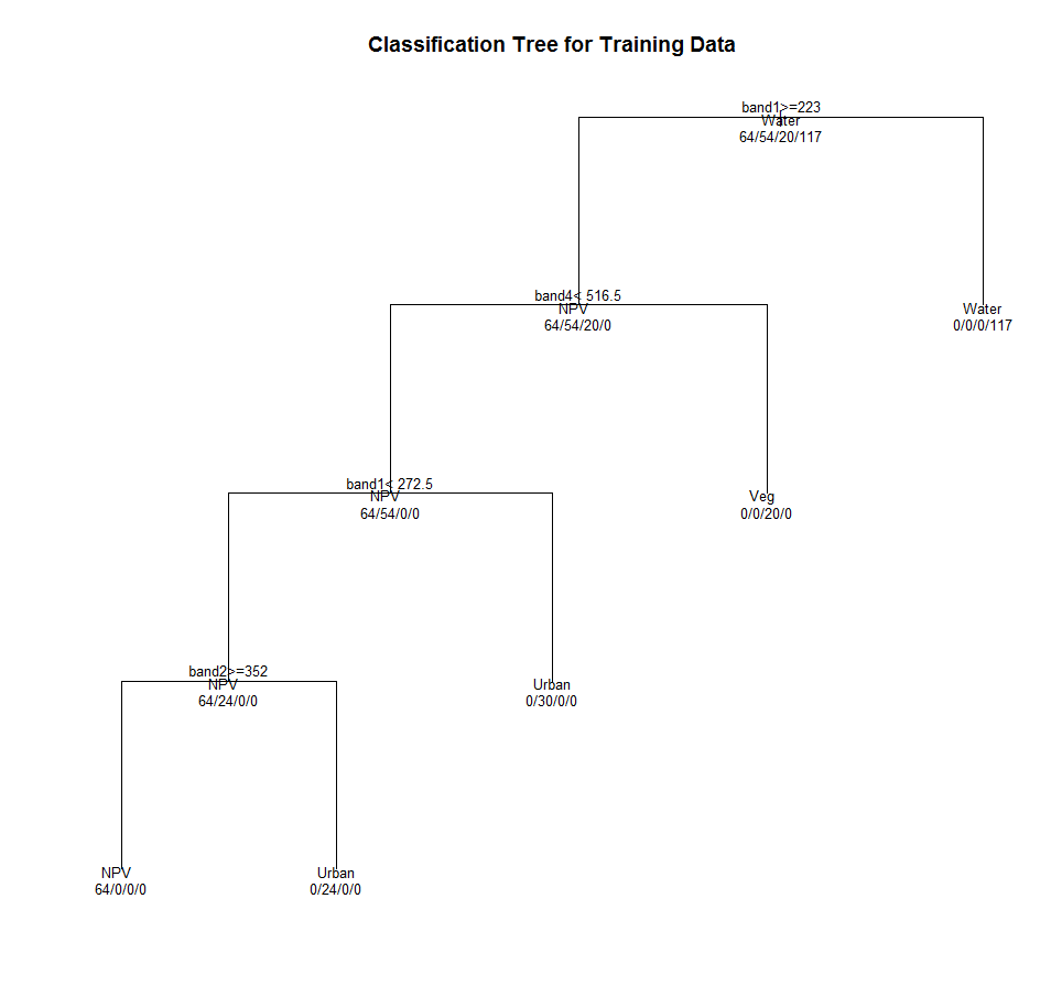
To begin with, I simply pulled up some data, subsetted it and did a manual classification on the data.  I chose 4 different classes: NPV, VEG, Urban, and Water.

;Start ENVI

e = envi(/current)

if ~OBJ_VALID(e) then e = envi()

 

; Open the test image

file1 = FILEPATH('qb_boulder_msi', ROOT_DIR=e.ROOT_DIR, $

  SUBDIRECTORY = ['data'])

oRaster = e.OpenRaster(file1)

 

; Subset the image

oSubSet = oRaster.Subset(Sub_Rect = [207,705,420,838])

 

; Get the offset for the imagery

xo = oSubset.METADATA['X START']

yo = oSubset.METADATA['Y START']

 

; Pullout the ROI Data

Water = oSubset.GetData(Sub_Rect = [300-xo,800-yo,312-xo,808-yo], interleave='bip')

NPV = oSubset.GetData(Sub_Rect = [242-xo,758-yo,249-xo,765-yo], interleave='bip')

Urban1 = oSubset.GetData(Sub_Rect = [321-xo,736-yo,326-xo,740-yo], interleave='bip')

Urban2 = oSubset.GetData(Sub_Rect = [363-xo,713-yo,366-xo,718-yo], interleave='bip')

Veg = oSubset.GetData(Sub_Rect = [369-xo,738-yo,372-xo,742-yo], interleave='bip')

roi_data = list(Water,NPV,Urban1,Urban2,Veg)

I then structured the data in a way that allows for easier ingestion into the R environment.

; Get the size of the output array

npts = 0

for i = 0 , n_elements(roi_data)-1 do npts = npts + product((size(roi_data[i], /DIMENSIONS))[1:2])

training_data = intarr(oSubSet.nb,npts)

class = strarr(npts)

classes = ['Water', 'NPV', 'Urban', 'Urban', 'Veg']

 

;build the training data

count = 0

for i = 0 , n_elements(roi_data)-1 do begin

  training_data[*, count : count + product((size(roi_data[i], /DIMENSIONS))[1:2])-1] = reform(roi_data[i], oSubSet.nb, product((size(roi_data[i], /DIMENSIONS))[1:2]))

  class[count : count + product((size(roi_data[i], /DIMENSIONS))[1:2])-1] = classes[i]

  count = count + product((size(roi_data[i], /DIMENSIONS))[1:2])

endfor

 

; Collect the input info

classes = strjoin(class,",",/SINGLE)

band1 = training_data[0,*]

band2 = training_data[1,*]

band3 = training_data[2,*]

band4 = training_data[3,*]

Next comes the tricky part.  I called the rpy2 object from inside python and returned the robject to IDL.

; Get Python ready for the new R DataFrame

!null = Python.run('import rpy2.robjects as robjects')

robjects = Python.robjects

Once I had R all ready to go within Python, I wrote some simple R code on the fly within IDL that would allow me to visualize the different band thresholds that made up my manual image classification.

; Define the R function

train_rf = "robjects.r('''" + $

  "train_rf <- function(band1, band2, band3, band4, classes) { \n" + $

  "require(rpart) \n" + $

  "classes = c(unlist(strsplit(classes,','))) \n" + $

  "train_df = data.frame(band1, band2, band3, band4, classes) \n" + $

  "fit = rpart(classes ~ band1 + band2 + band3 + band4, method='class', data=train_df) \n" + $

  "plot(fit, uniform = TRUE, main = 'Classification Tree for Training Data') \n" + $

  "text(fit, use.n=TRUE, all=TRUE, cex=.8) \n" + $

      "}" + $

       "''')"

One possible hang-up here is that R must have the rpart package installed in order for this code to run. I installed this in the main R library directory to make sure that any user on my machine could find this package (i.e. C:\Program Files\R\R-3.1.3\library). As long as this package has been installed the “require(rpart)” portion of the code should not give you any trouble. 

Finally, you will need to publish the newly defined train_rf function up to Python.

!null = Python.run(train_rf)

 

Once it has been recognized by Python, you can bring it into IDL and run it as if it were a native function.

train_rf = robjects.globalenv['train_rf']

 

; Call the r function from within IDL

result = train_rf(band1, band2,Band3, band4, classes)

When you run the code, it should generate something that looks like this!