Customizing Mouse Handler for IDL 8 Graphics Windows
Anonym
This blog post provides an example program that addresses some questions that we have received in Tech Support in the past few weeks. The example code contains two routines (“ex_closest_xy_widget” and “closest_wid_mouse_down” ) and is shown at the bottom of this post.
The main problems that are addressed in this example program are:
- Given a data set with various X an Y values, if you are given a separate set of X0 and Y0 coordinates, how do you determine which data point is closest to these coordinates?
- How do you create a quick interactive GUI to display the information from problem (1) with IDL 8 Graphics?
- How can you adjust the LEGEND object to only show one symbol?
A solution to problem (1) is to calculate differences between X and X0 and Y and Y0 for each data point in the data set. Then, calculate the magnitude of these differences and find the minimum value. Since IDL is a vectorized, this can be performed in a couple lines of code:
d = sqrt((x-(x0))^2+(y-(y0))^2)
imin = where(d eq min(d))
IDL 8 Graphics (aka New Graphics, aka Function Graphics) are interactive, and you can customize the event handlers of the graphics' windows. Therefore, you use IDL 8 Graphics to generate pretty good GUI applications without building a widget from scratch. Thus, a solution to the problem (2) is to generate a scatter plot with the original data and then customize the MOUSE_DOWN_HANDLER to allow the user to select “target” coordinates in the plot, then you can use the solution to problem (1) to find the closest data point and display this information.
Finally, if you try to make a legend for a plot with symbols using the LEGEND function, you will find that by default that it displays a symbol three times. If you want to change the legend to only display the symbol once, you can do this by setting the SAMPLE_WIDTH property to 0 (the three symbols are still generated but are right on top of one another). However, this may cause the symbols to appear outside the boarder of the legend. To fix this problem, you can adjust the HORIZONTAL_SPACING keyword. A sample of code that shows how this can be done is shown below:
lgnd = legend(target=[p,p0, p1], $
sample_width=0, $
horizontal_spacing=.1, $
/auto_text_color)
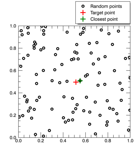
The example routines “closest_wid_mouse_down” and “ex_closest_xy_widget” are shown below. I would like to thank my colleague Jim Uba who contributed heavily to the code below, and figured out the LEGEND trick discussed previously. After you have run this code, left click in the window, and it should display a plot that is similar to the following:
function closest_wid_mouse_down, owin, x0, y0, button, keymods, clicks
compile_opt idl2
if (button eq 1 ) then begin ;only perform on left mouse click
;get the state variable from the plot window
state = owin.uvalue
;get the reference to the random data point
p = state['p']
;the x and y points returned by the mouse
;handler are in device coordinates by default
;use the convertcoord method to convert it
;to data coordinates
data_coord = p.convertcoord(x0,y0,/device, /to_data)
x0 = data_coord[0]
y0 = data_coord[1]
state['x0']=x0
state['y0']=y0
;get the reference to the "closest point" scatter plot
p1 = state['p1']
;get the reference to the "selected point" scatter plot
p0 = state['p0']
;get the data
x = state['x']
y = state['y']
; calcuate the distances from the data
; points to the target point
d = sqrt((x-(x0))^2+(y-(y0))^2)
; find the array index of the xy point
; with minimum distance to the target point.
imin = where(d eq min(d))
;change the data of the "selected point" scatter plot
;to the point selected by the user. set hide=0 to make
;sure data displays correctly
p0.setdata, [x0,x0],[y0,y0]
p0.hide=0
;change the data of the "selected point" scatter plot
;to the point selected by the user
p1.setdata, [x[imin],x[imin]], [y[imin],y[imin]]
p1.hide=0
;print the selected point
print, "selected point:"
print, "x: ", x0
print, "y: ", y0
;print the closest point
print, "closest data point:"
print, "x: ", x[imin]
print, "y: ", y[imin]
endif
return, 1
end
pro ex_closest_xy_widget
; create random xy data points
x = randomu(seed, 100)
y = randomu(seed, 100)
;inital points to get the distance
x0 = 0
y0 = 0
;generate scatterplot of random xy points
p = scatterplot(x, y, $
sym_color='black', symbol='o', $
sym_size=1, sym_thick=3, $
aspect_ratio=1, $
name='random points', uvalue='p')
;generate scatterplot of the selected point
;this plot isn't very useful at this time because
;the user hasn't selected a point. use hide keyword
;to hide it for now
p0 = scatterplot([x0,x0], [y0,y0], $
sym_color='red', symbol='+', $
sym_size=2, sym_thick=3, $
/current, /overplot, $
name='target point', /hide,uvalue='p0')
;generate scatterplot of the selected point
;this plot isn't very useful at this time because
;the user hasn't selected a point. use
p1 = scatterplot( [x[0],x[0]], [y[0],y[0]], $
sym_color='green', symbol='+', $
sym_size=2, sym_thick=3, $
/current, /overplot, $
name='closest point',/hide,uvalue='p2')
;generate a state variable to store information needed for the
;handler. note: using a hash is a really convenient way to do
;this because they are easy to generate and use, and the data is
;stored as heap memory
state=hash()
state['p'] = p
state['x'] = x
state['y'] = y
state['x0'] = x0
state['y0'] = y0
state['p0'] = p0
state['p1'] = p1
;assign the state variable as the uvalue of the
;scatterplot window
p.window.uvalue = state
;set the mouse_down_handler of the
;window to "closet_wid_mouse_down"
p.window.mouse_down_handler="closest_wid_mouse_down"
;generate a legend. by default this will generate 3
;symbols. if you make the sample_width=0, and adjust
;the horizontal_spacing, you can make the legend on
lgnd = legend(target=[p,p0, p1], $
sample_width=0, $
horizontal_spacing=.1, $
/auto_text_color)
;position the plot and legend in the window
p.position = [.54,.45]
lgnd.position=[.84,.99]
end