Spatial/Spectral Browsing and Endmembers
The Spectral Hourglass Series: Part 2
Anonym
Before jumping down the rabbit hole of the Spectral Hourglass Workflow we must define the concept of an endmember, for endmembers are at the core of hyperspectral data analysis. Along with endmembers, we will discuss atmospheric correction and the need to convert our data to apparent reflectance to pursue quantitative analysis down the road.
Endmembers are defined as materials that are spectrally unique in the wavelength bands used to collect the image — that is, endmember spectra cannot be reconstructed as a linear combination of other image spectra. It is often desirable to find the pixels in an image that are the purest examples of the endmember materials in the scene. These pixel spectra can then be used to map the endmember materials in various ways. Throughout this blog series we explore two ways to determine the pixels representing the purest examples of each endmember.
An alternative to extracting endmember spectra directly from the image is to use laboratory or field spectra of the materials of interest to define the target for mapping or classification. One disadvantage of this approach is that it requires comparing lab/field spectra with image spectra. Image spectra — even after calibration and atmospheric correction — often have remnants and artifacts caused by the sensor, solar curve, and/or atmosphere specific to the image. Moreover, lab/field spectra are typically collected from much smaller samples than the pixel size of the image. Image-derived endmember spectra will therefore be more comparable with other pixel spectra in the image. Consequently, using image-derived endmember spectra to define the materials of interest can often lead to better results when looking for those materials of interest throughout the image.
This brings us to the first step in the Spectral Hourglass Workflow. Spatial/Spectral Browsing Preprocessing for nearly all raster images includes use of the same two initial steps: Radiometric Calibration and Atmospheric Correction. Beyond these preprocessing steps you may desire to orthorectify an image, or perhaps mosaic the image. However, these first two steps are required if you wish to perform quantitative analysis later on.
ENVI offers several different tools to convert your data to apparent reflectance: Dark Object Subtraction, Quick Atmospheric Correction (QUAC), and Fast-Line-of-sight Atmospheric Analysis of Spectral Hypercubes (FLAASH). You can tell by the name that FLAASH has been developed specifically for hyperspectral data; FLAASH is a sophisticated radiative transfer program that converts both multispectral and hyperspectral data to reflectance. It incorporates the MODTRAN radiation transfer code, modeling atmospheric properties and the solar irradiance curve. Water vapor amounts are calculated on a pixel-by-pixel basis using either the 1135, 940, or 820 nm absorption.
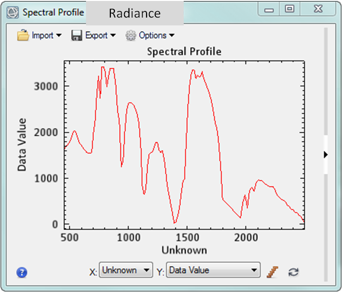
Spectral Profile of Radiance Data
Spectral Profile of Reflectance Data
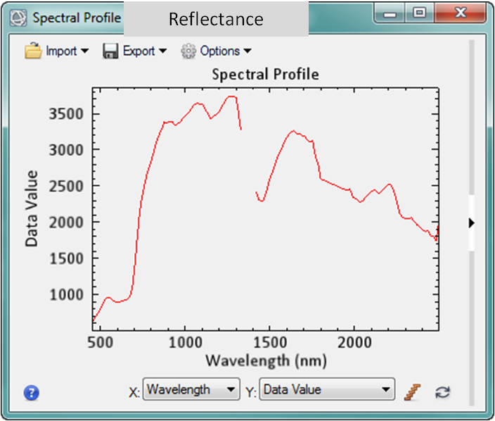
We convert to apparent reflectance in an effort to remove atmospheric absorption, scattering effects, and the solar irradiation curve. Theoretically, the concept of apparent reflectance states that we are viewing the reflectance of the data found on the surface of the earth, not through layers of atmosphere all the way up to the sensor. In essence, the spectra of each pixel will more accurately represent the surface of the earth that the pixel represents. As we extract our endmembers later in the workflow, we can compare them to library spectra and identify materials with similar spectral angles, allowing us to identify materials in the scene and estimating their total abundance.
Note that we will need to apply a scale factor when comparing our in-scene spectra to our library spectra, due to the controlled nature of laboratory spectra. Unlike our in-scene spectra that is collected using the passive light source of the sun, laboratory spectra are collected with an active light source that does not alter in intensity. Our in-scene data fluctuation will be much more drastic by comparsion.
Once you have completed this first step within the Spectral Hourglass Workflow, it is wise to explore the image and the associated spectra within each pixel to detect the presence of man-made materials, minerals, vegetation, etc. found throughout your scene.
The next part of the blog series will focus on reducing the dimensionality of the dataset and how to separate signal from noise in our data.
Read The Spectral Hourglass Series: Part 3, Hyperspectral Data Reduction
Read The Spectral Hourglass Series: Part 1, An Introduction