How to Create a Buffered Line Graph
The following example code example demonstrates how to create a line graph with a buffer. This requires the use of the FILL_LEVEL property in conjunction with the FILL_BACKGROUND property. The FILL_LEVEL is the Y-value for the boundary below the plot line. Setting the FILL_BACKGROUND creates the fill underneath the line plot.
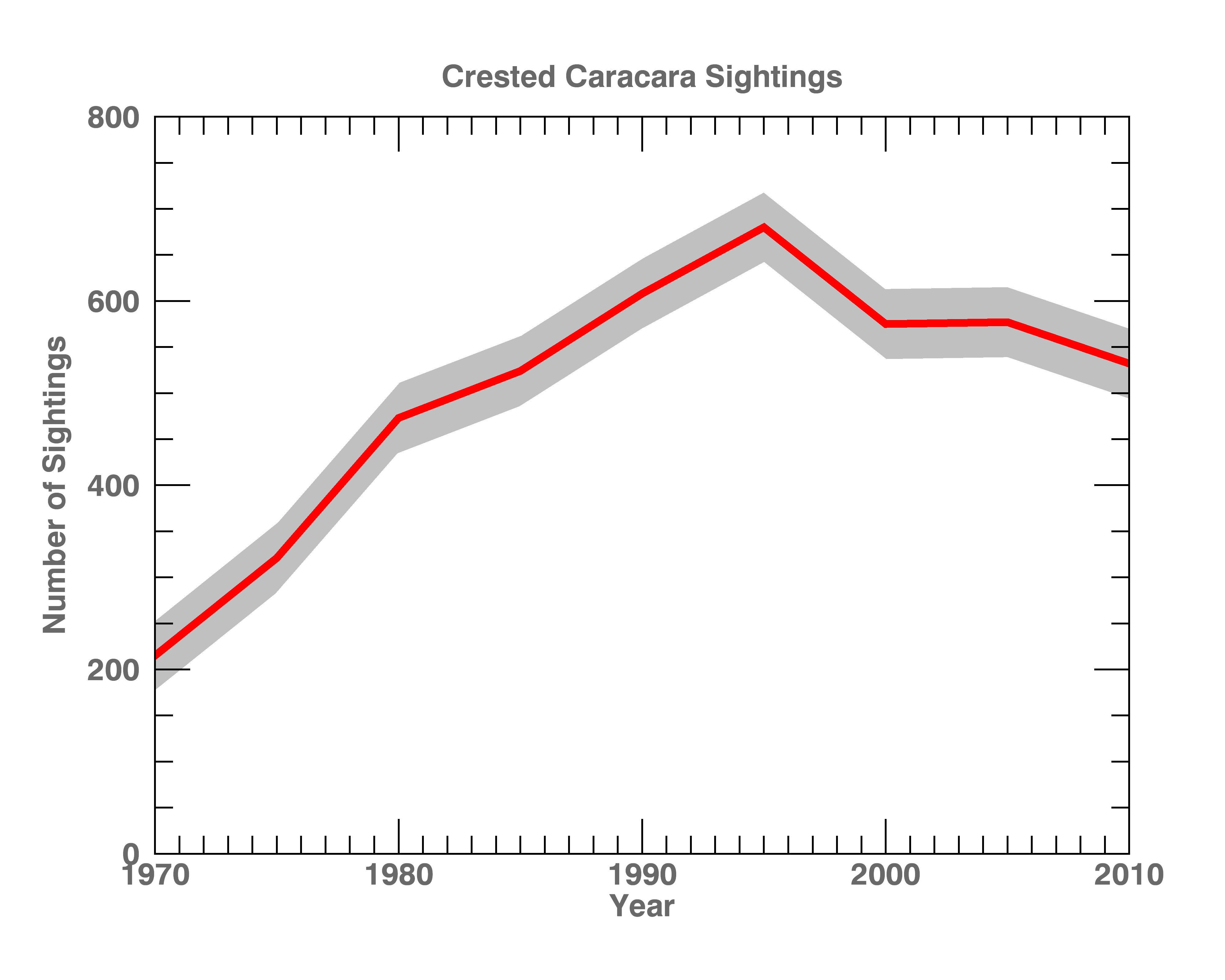
In this example the first line, which is the upper buffer limit, uses the gray color for its fill. This is also the buffer colour. The second line is the lower buffer line and its fill colour is white and overlays the gray creating the desired width. The final line is the actual data line and is overplotted on the other plots.
pro ex_shaded_region_plot
; Define the data. The data in this example are called sightings.
year = [1970, 1975, 1980, 1985, 1990, 1995, 2000, 2005, 2010]
sightings = [215, 321, 473, 524, 608, 680, 575, 577, 532]
; Add desired buffer widths to the 'sightings' line
sightings_up40= sightings + 40
sightings_down40= sightings - 40
;Since 'fill_level' goes down calculate the lowest potential value
;from this line which is the upper buffer edge.
p2=plot(year,sightings_up40, thick=2, fill_level=175.0, $
color='white', $ ; to create clean buffer line
fill_background=1, $
fill_color='silver')
;Set the 'fill_level' to a value that is lower than value for 'p2'. The overplot covers the
;silver color from p2 with white (to blend with background).This becomes the lower buffer edge.
p3=plot(year,sightings_down40,thick=2, fill_level=100.0, $
color='white', $ ; to create clean buffer line
fill_background=1, fill_color='white',/overplot)
;Now overplot the orginal line...
p1=plot(year,sightings,thick=4, color='red',$
title='Crested Caracara Sightings',$
xtitle='Year', $
ytitle='Number of Sightings', $
font_style= 'bold', $
font_color= 'dim gray', $
/overplot)
END