Using Attributes to Improve Image Classification Accuracy

In this article I will show an example of how you can improve the accuracy of a supervised classification by considering different attributes.

Supervised classification typically involves a multi-band image and ground-truth data for training. The classification is thus restricted to spectral information only; for example, radiance or reflectance values in various wavelengths. However, adding different types of data to the source image gives a classifier more information to consider when assigning pixels to classes.

Attributes are unique characteristics that can help distinguish between different objects in an image. Examples include elevation, texture, and saturation. In ENVI you can create a georeferenced layer stack  image where each band is a separate attribute. Then you can classify the attribute image using training data.

Creating an attribute image is an example of data fusion in remote sensing. This is the process of combining data from multiple sources to produce a dataset that contains more detailed information than each of the individual sources.

Think about what attributes will best distinguish between the different classes. Spectral indices are easy to create and can help identify different features. Vegetation indices are a good addition to an attribute image if different vegetation types will be classified.

Here are some other attributes to experiment with:

• Texture measures (occurrence and co-occurrence)
• Synthetic aperture rader (SAR) data
• Color transforms (hue, saturation, intensity, lightness)

Including elevation data with your source imagery helps to identify features with noticeable height such as buildings and trees. If point clouds are available for the study area, you can use ENVI LiDAR to create digital surface model (DSM) and digital elevation model (DEM) images. Use Band Math to subtract the DEM from the DSM to create a height image, where pixels represent absolute heights in meters. In the following example, the brightest pixels represent trees. You can also see building outlines.

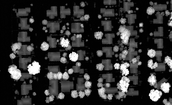
Example height image at 1-meter spatial resolution

Locating coincident point cloud data for your study area (preferably around the same date) can be a challenge. Luckily I found the perfect set of coincident data for a classification experiment.

Example

The National Ecological Observatory Network (NEON) provides field measurements and airborne remote sensing datasets for terrestrial and aquatic study sites throughout the world. Their Airborne Observation Platform (AOP) carries an imaging spectrometer with 428 narrow spectral bands extending from 380 to 2510 nanometers with a spectral sampling of 5 nanometers. Also onboard is a full-waveform LiDAR sensor and a high-resolution red/green/blue (RGB) camera. For a given observation site, the hyperspectral data, LiDAR data, and high-resolution orthophotography are available for the same sampling period.

I acquired a sample of NEON data near Grand Junction, Colorado from July 2013. My goal was to create an urban land-use classification map using an attribute image and training data. For experimentation and to reduce processing time, I only extracted the RGB and near-infrared bands from the hyperspectral dataset and created a multispectral image with these bands. I used ENVI LiDAR to extract a DEM and DSM from the point clouds. Then I created a height image whose pixels lined up exactly with the multispectral image.

I created an Enhanced Vegetation Index (EVI) image using the Spectral Indices tool. Finally, I combined the RGB/NIR images, the relative height image, and the EVI image into a single attribute image using the Layer Stacking tool.

Next, I used the Region of Interest (ROI) tool to collect samples of pixels from the multispectral image that I knew represented five dominant classes in the scene: Water, Asphalt, Concrete, Grass, and Trees. I used a NEON orthophoto to help verify the different land-cover types.

I ran seven different supervised classifiers with the multispectral image, then again with the attribute image. Here are some examples of Maximum Likelihood classifier results:

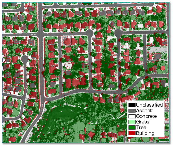
Maximum Likelihood classification result from the NEON multispectral image

Notice how the classifier assigned some Building pixels to Asphalt throughout the image. 

Here is an improved result using the attribute image. Those pixels are correctly classified as Building now.

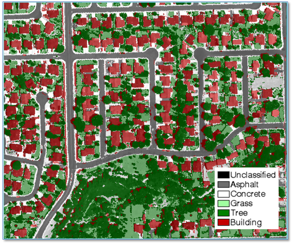
Maximum Likelihood classification result using the attribute image

A confusion matrix and accuracy metrics can help verify the accuracy of the classification.

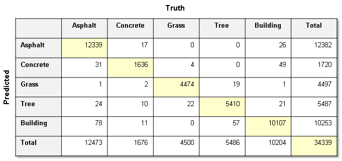
Confusion matrix calculated from the attribute image classification

The following table shows how the Overall Accuracy value is higher with the attribute image when using different supervised classifiers:

	Multispectral image	Attribute Image
Mahalanobis Distance	72.5	83.8
Minimum Distance	57.69	95.22
Maximum Likelihood	91.3	98.91
Parallelepiped	57.18	95.8
Spectral Angle Mapper	54.97	61.79
Spectral Information Divergence	62.1	66.93
Support Vector Machine	85.03	99.16

 

The accuracy of a supervised classification depends on the quality of your training data as well as a good selection of attributes. In some cases, too many attributes added to a multispectral image can make the classification result worse, so you should experiment with what works best for your study area. Also, some classifiers work better than others when considering different spatial and spectral attributes. Finally, you may need to normalize the different data layers in the attribute image if their pixel values have a wide variation.

New tutorials will be available in ENVI 5.4 for creating attribute images and for defining training data for supervised classification.

 

Resources

National Ecological Observatory Network. 2016. Data accessed on 28 July 2016. Available on-line at https://www.neonscience.org from National Ecological Observatory Network, Boulder, CO, USA.