When Should I Correct My Imagery for Atmospheric Effects?
Anonym
This is one of the most frequently asked questions that we receive, especially from those who are getting started in remote sensing. The answer depends on the particular application and sensor, but in general you should apply remote sensing atmospheric correction before doing any spectral analysis with optical imagery. In this article I will give some guidelines on when to apply atmospheric correction and the best methods for each application.
Atmospheric correction of optical imagery typically means removing the effects of clouds and aerosols from a radiance image. The result is an apparent surface reflectance image, which can be used to extract accurate spectral information from features on the Earth's surface.
You can also calibrate imagery from some sensors to top-of-atmosphere (TOA) reflectance if sufficient metadata are available. See the article Digital Number, Radiance, and Reflectance for more information. Is it sufficient to calibrate an image to TOA reflectance without going through the process of creating a surface reflectance image? Look at the following WorldView-3 images, courtesy of DigitalGlobe. Both images were scaled from 0 to 1 in units of reflectance, and both are displayed with a 1% linear stretch:
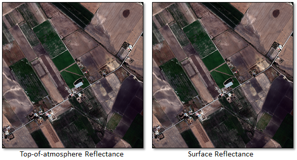
They are visually identical because only the RGB bands are displayed. However, a spectral plot of a single pixel reveals differences between the two images:
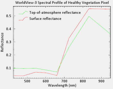
This difference illustrates the importance of removing atmospheric effects from a calibrated image. Here, the surface reflectance curve more accurately represents the characteristics of healthy vegetation with a steeper red edge curve near 700 nanometers, compared to the TOA reflectance curve. This highlights the role of remote sensing atmospheric correction in producing reliable data.
Next, we will look at more specific applications.
Classification and Change Detection
In general, atmospheric correction is unnecessary prior to unsupervised image classification or change detection. Chinsu et al. (2015) suggest that atmospheric correction will not improve the accuracy of results in land use and land cover (LULC) classification.
An article by Song et al. (2011) provides more detailed guidelines, suggesting that correction is unnecessary in classification and change detection except when training data from one time or place are applied in a different time or place. Even then, a dark subtraction method is often sufficient.
For supervised image classification, if you use spectral signatures from a spectral library as endmembers or training samples, atmospheric correction is usually required. This is because spectral libraries collected from the field uses surface reflectance.
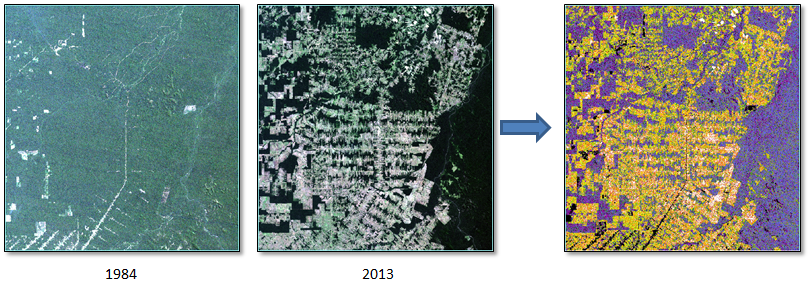
Image difference change detection between a Landsat TM image (1984) and Landsat-8 image (2013) of the Amazon rain forest. This process required radiometric normalization but no atmospheric correction.
Spectral Indices
Calibrating imagery to apparent surface reflectance yields the most accurate results with spectral indices. This is especially important for hyperspectral sensors. It also ensures consistency when comparing indices over time and from different sensors.
Some vegetation indices such as NDVI are more sensitive to atmospheric effects than others. For example, the Atmospherically Resistant Vegetation Index (ARVI) and related indices such as GARI and VARI were designed to minimize the effects of atmospheric scattering in the blue wavelengths. Atmospheric correction is unnecessary with these indices.
When using multispectral imagery (e.g., Landsat TM) to compute spectral indices, a simple method such as QUAC® or dark subtraction may be sufficient to account for atmospheric effects (Hadjimitsis et al., 2015). Some may prefer a more rigorous, model-based method such as FLAASH®. These tools are part of the ENVI Atmospheric Correction Module and should be used with super-spectral imagery such as WorldView-3, and with hyperspectral imagery.
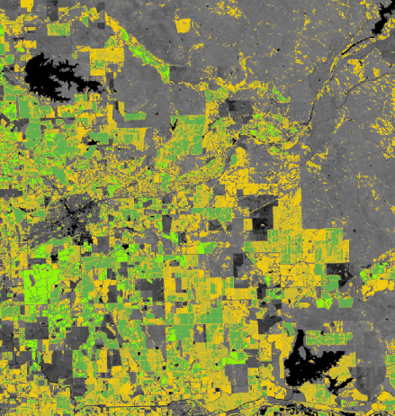
Green Vegetation Index (GVI) image created from a Landsat-8 scene of the Central Valley, California, 21 May 2015. The original scene was calibrated to spectral radiance, then QUAC atmospheric correction was applied before computing GVI.
Material Identification
Hyperspectral and super-spectral sensors are used for applications such as material identification. When analyzing imagery from multispectral sensors such as Landsat TM or GeoEye, atmospheric effects are of a lesser concern because the channels are designed to accomodate atmospheric gas absorption features. However, hyperspectral and super-spectral sensors cover all of the visible and near-infrared spectrum, including absorption features.
You can use QUAC or FLAASH to remove the effects of atmospheric scattering and gas absorption to produce surface reflectance data. See the Preprocessing AVIRIS Data Tutorial for an example.
QUAC is simple to use and produces accurate results in the following conditions:
- The scene must have several diverse materials; QUAC will not work well in a homogenous scene.
- Pixels of ocean or large water bodies should be masked out first.
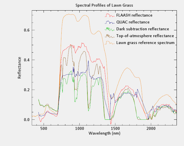
The following plot compares reflectance values of different correction methods for a single pixel of healthy vegetation from an EO-1 Hyperion image. The two most rigorous methods--QUAC and FLAASH--create reflectance profiles that more accurately represent healthy vegetation. The absorption features of FLAASH and QUAC results are closer to the reference spectrum, compared to dark subtraction and TOA reflectance.
Many good resources are available that explain atmospheric correction in more detail. This article only touched on the subject, but hopefully you have some tips to get you started.
References
Chinsu, L., C.C. Wu, K. Tsogt, Y.C. Ouyang, and C.I. Chang. “Effects of AtmosphericCorrection and Pansharpening on LULC Classification Accuracy Using WorldView-2 Imagery.” Information Processing in Agriculture 2 (2015): 25-36.
Hadjimitsis, D.G., G. Papadavid, A. Agapiou, K. Themistocleous, M.G. Hadjimitsis, A. Retalis, S. Michaelides, N. Chrysoulakis, L. Toulios, and C.R .I. Clayton. “Atmospheric Correction for Satellite Remotely Sensed Data Intended for Agricultural Applications: Impact on Vegetation Indices.” Natural Hazards and Earth Systems Sciences 10 (2010): 89-95.
Song, C., C. Woodcock, K. Seto, M.P. Lenney, and S. Macomber. “Classification and Change Detection Using Landsat TM Data: When and How to Correct Atmospheric Effects?” Remote Sensing of Environment 75 (2001): 230-244.