This tutorial demonstrates how to calibrate an AVIRIS image to surface reflectance, while teaching the following concepts:
- Why you should preprocess hyperspectral data
- How to use FLAASH to correct for atmospheric effects
- How to plot radiance and reflectance spectra
- How to remove bad bands from reflectance data, which removes artifacts from the plotted spectra.
You must have a separate license for the Atmospheric Correction Module: QUAC and FLAASH to use this tutorial.
This is the first in a series of tutorials that demonstrate how to work with hyperspectral data. Here are the other tutorials:
Files Used in this Tutorial
Tutorial files are available from our ENVI Tutorials web page. Click the Hyperspectral link to download the .zip file to your machine, then unzip the files.
The image used in this exercise was collected by the Airborne Visible Infrared Imaging Spectrometer (AVIRIS) sensor. AVIRIS data files are courtesy of NASA/JPL-Caltech. The sample image covers the Cuprite Hills area of southern Nevada, an area with diverse mineral types. The scene was collected from an ER-2 aircraft on August 8, 2011. The full original scene is available from NASA/JPL.
|
File |
Description |
|
CupriteAVIRISSubset.dat
|
AVIRIS radiance image and header file, spatially subsetted and saved to ENVI image format.
|
|
AVIRIS11_gain.txt
|
Text file with multiplication factors used for calibration to spectral radiance
|
Background
Hyperspectral sensors, also called imaging spectrometers, should be spectrally and radiometrically calibrated before you analyze their data. NASA/JPL has already processed the AVIRIS data to remove geometric and radiometric errors associated with the motion of the aircraft used during data collection. However, the data should be further corrected for atmospheric effects and converted to surface reflectance prior to scientific analysis. Before you begin the tutorial, you should understand some basic concepts about the different types of information stored in the pixel values of your imagery.
Raw DN Data
Pixel values are also called digital numbers, or DN values. They have not yet been calibrated into physically meaningful units; they are 2-byte (16-bit) signed integer data that include the effects of surface reflectance, the solar irradiance curve, scattering, atmospheric gas absorptions, variation in illumination due to topography, and instrument response.
Radiance
Radiance is the amount of radiation coming from an area. It includes radiation reflected from the surface, from neighboring pixels, and from clouds. Calibration to radiance compensates for variations in detector sensitivity. To derive a radiance image from an uncalibrated image, you must multiply the raw data by a series of gain values, one for each band. Resulting pixel values are typically in units of W/(m2 * sr * µm).
Data vendors usually provide gains/offsets in the metadata that accompanies the imagery. NASA/JPL documented the gain values for 2011 AVIRIS data in the file AVIRIS11_gain.txt, which you will use later in this tutorial. By applying the gains from this file, the AVIRIS radiance image will be in units of µW/(cm2 * sr * nm). This image uses specialized gain values retrieved when the image was downloaded. FLAASH defaults to an input scale of 1, which is used by all AVIRIS-NG images.
Radiance images include the radiation effects of the sun; in fact, a spectrum of a radiance pixel closely matches that of the solar irradiance curve, also called the solar spectrum. For hyperspectral data analysis, you should remove the effects of solar irradiance by calibrating the data to reflectance.
Reflectance
Reflectance is the proportion of the radiation reflected off a surface to the radiation striking it. In hyperspectral data analysis, materials are identified by their reflectance spectra. So calibrating the data to reflectance is the first step toward identifying materials from an image. When analyzing imagery from multispectral sensors (such as Landsat or GeoEye), atmospheric effects are of lesser concern because the channels are designed to accommodate atmospheric gas absorption features. However, hyperspectral sensors cover all of the visible and near-infrared spectrum, including absorption features. So it is important to compensate for these effects in hyperspectral imagery.
Other advantages of using reflectance data include:
- Spectral features are more apparent in the imagery
- The shape of the image spectra are mostly influenced by chemical and physical properties of the surface materials, rather than by atmospheric and solar effects.
An atmospheric correction tool such as FLAASH can remove the effects of atmospheric scattering and gas absorptions to produce reflectance data. With hyperspectral data analysis, calibrating imagery to apparent surface reflectance is sufficient; the imagery may still have variations in illumination due to topography. With reflectance data, pixel values typically range from 0 to 1 but are often scaled by some factor to yield integer data. FLAASH automatically scales reflectance values by 10,000.
We will demonstrate these concepts in the steps that follow.
Display the Uncorrected Data
- Start ENVI.
- From the menu bar, select File > Open and select the file CupriteAVIRISSubset.dat. ENVI displays the image with an approximate true-color representation.
- Double-click the filename in the Layer Manager to open the Metadata Viewer. Here, you can see more information about the file. For example:
- Click the Map Info category to see the pixel size and units.
- Click the Extents category to see the geographic coordinates of the spatial extent.
- Click the Spectral category to see the wavelengths defined for each of the 224 bands. The FWHM column lists the full-width-half-maximum values that NASA/JPL provided for the AVIRIS file.
- Click the Close button to close the Metadata Viewer.
-
In the middle of the Status bar (at the bottom of the application), right-click and select Raster Data Values. When you move the cursor around the image, the Status Bar shows the pixel values for the red, green, and blue channels. These are 2-byte signed integer data.
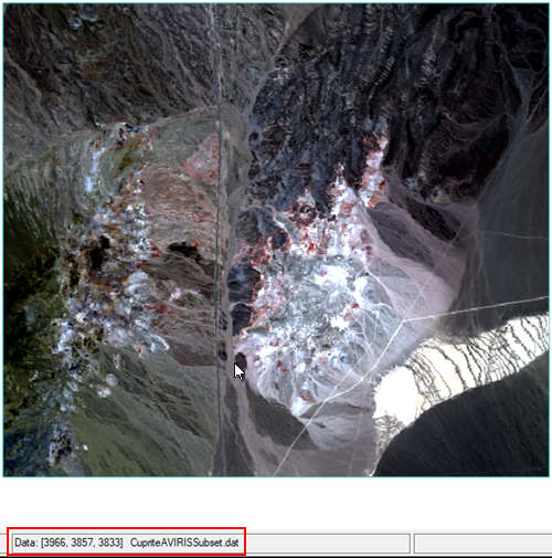
- In the Layer Manager, right-click on layer name and select Profiles > Spectral.
- Click inside of the image to move the crosshairs to a different location. The Spectral Profile dialog updates with the spectrum of that pixel location. Notice how the shape of the radiance curve changes slightly as you move the crosshairs to different materials within the scene.
The spectral profile, in general, shows some of the common atmospheric features often seen in hyperspectral data:
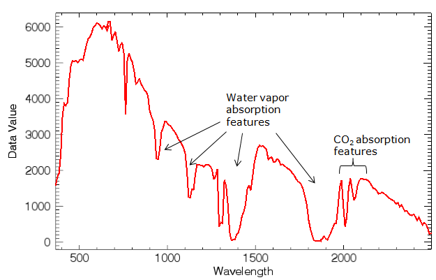
The FLAASH tool that you will use next will convert the radiance data to reflectance.
Start FLAASH
FLAASH is a model-based radiative transfer program to convert radiance data to reflectance.
To run FLAASH, you must purchase a separate license for the Atmospheric Correction Module: FLAASH and QUAC from NV5 Geospatial Solutionssales representative.
- In the Toolbox search field, type flaash. Double-click on the FLAASH Atmospheric Correction tool name. The Data Selection dialog appears.
- Select the file CupriteAVIRISSubset.dat, and click OK. The FLAASH - Rigorous Atmospheric Correction dialog appears, with the Main tab selected.
Set Time and Output Options
- Use the Acquisition Date/Time drop-down lists to set the date to 6 August 2011 and the flight time to 19:20:00.
- In the Output Raster field, specify the path and filename you want to write the output reflectance image to. Type CupriteReflectance.dat. Disable the Display result check box.
Select Sensor and Geometric Options
- Select the Sensor tab in the FLAASH dialog. From the Sensor Type drop-down button, select Hyperspectral > AVIRIS.
-
For the Input Scale, import the values from AVIRIS11_gain.txt file. Click the Load Values button  , navigate to the file, and click Open.
The scale factors in this file boost the signal from each channel, especially in the shortwave-infrared spectrum where the solar irradiance signal is much lower. This results in higher levels of radiance. In this particular file, Bands 1-110 have a scale factor of 300, Bands 111-160 have a scale factor of 600, and Bands 161-224 have a scale factor of 1200. When each spectrum is divided by the factors in this file, the 16-bit integers will be converted to radiance in units of µW/(cm2 * sr * nm).
- Select the Geometric tab. Set the Sensor Altitude to 20.
- Set the Ground Elevation to 0.6
The Sensor Altitude field is typically 20 km for the ER-2 aircraft collecting AVIRIS data. The Ground Elevation value was estimated using Google Earth. (Another option is to view the GMTED2010 DEM file that is installed with ENVI.) The flight date and time were recorded in an *.info file that NASA/JPL provided with the AVIRIS imagery.
While more accurate values are best, none of the fields require precise data. They are only used to determine the approximate geographic location and solar elevation angle at the scene, for the atmospheric correction model.
Select Atmospheric Model, Water, and Arerosol Options
Hyperspectral images typically include enough spectral information needed to estimate water vapor and aerosols in the atmosphere. You will set parameters to retrieve water vapor and aerosols in the following steps.
- Select the Model tab. From the Atmospheric Model drop-down button, select 1975 US Standard Atmposphere.
- Select the Water tab. From the Water Absorption Wavelength drop-down list, select 1130. If you select 1130 nm or 940 nm and the feature is saturated due to an extremely wet atmosphere (unlikely for summer in southern Nevada), then use the 820 nm setting instead.
- Select the Aerosol tab. Keep the default value of High-Visibility Rural for Aerosol Model. This is a good option for the location of this scene in southern Nevada, where aerosols are not strongly affected by urban or industrial sources. The choice of model actually is not critical in this case, as the visibility is typically greater than 40 km.
- Click OK.
Display the Reflectance Image
- From the menu bar, select File > Open.
- Navigate to the output folder for FLAASH files, and select CupriteReflectance.dat. Click Open.
- Click the Data Manager button
 in the toolbar.
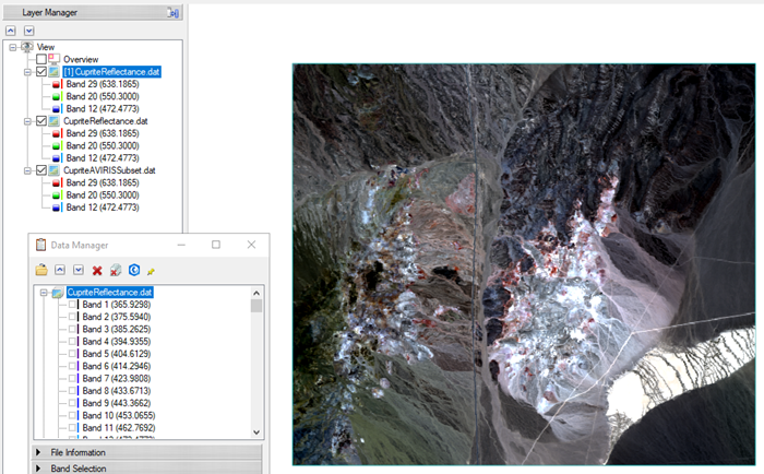
- Scroll down the list of files until you come to CupriteReflectance.dat.
-
Right-click on CupriteReflectance.dat, and select Load True Color. The reflectance image appears in the display.
- With the radiance and reflectance images both selected in the Layer Manager, click the Cursor Value button
 in the toolbar.
- The On demand updates button
 in the Cursor Value dialog is enabled by default. Click it to turn off the red probe.
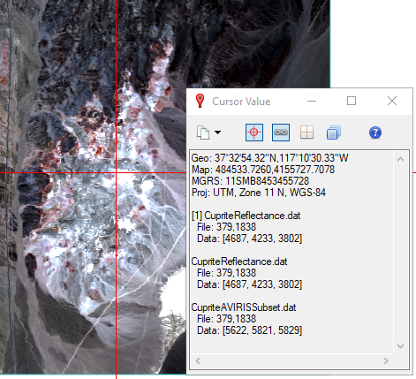
-
Move the cursor around the display, and compare data values from both images. The following screen capture shows an example of a pixel location over a black area of the image. Look for the "Data" row in each image.
-
Close the Cursor Value dialog.
FLAASH automatically scaled the reflectance values by 10,000. In this example, the pixel value for the red band of the reflectance image is 2031, or 0.2, if divided by 10,000. Reflectance values range from 0 to 1.0.
View Spectral Profile
- Click the Spectral Profile button
 in the toolbar.
- Click anywhere in the image. The Spectral Profile shows the spectrum for the selected pixel location.
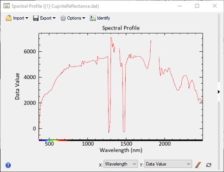
Note the shape of the reflectance curve and how it generally peaks near 1400 nanometers (nm). FLAASH determined that some bands were "bad" according to the strength of the reflectance signal, and the pixel values from these bands were omitted from the spectral profile. These appear as gaps in the reflectance curve. FLAASH wrote these bad bands to the ENVI header file that accompanies the reflectance image. In the header file, bad bands are indicated by a 0 under the bbl field. Reviewing the header file shows that Bands 108-112 and 155-166 were designated as bad.
-
In the Go To field in the toolbar, enter pixel coordinates 412,1880 and press the Enter key. Note the reflectance curve for this pixel location: it has two spikes centered over 1300 nm and 1500 nm:
Conversion of radiance data to reflectance using a model-based program such as FLAASH can introduce artifacts into the spectra. These artifacts can result from any of the following factors:
- Mismatches in the spectral calibration of the hyperspectral data set and the spectral radiative transfer calculations
- Errors in the absolute radiometric calibration
- Errors in the radiative transfer calculations
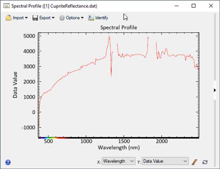
In addition, the 1400 nm and 1900 nm water vapor bands typically give very noisy reflectance results. These noisy values result from the low radiance values in these portions of the spectrum and can cause undesirable spikes. The following plot shows an example of this:
FLAASH attempts to correct for these artifacts by applying an EFFORT-based spectral polishing method on the data, if you set the Spectral Polishing toggle button to Yes. But it does not correct every artifact, especially with the noisy water vapor bands.
You can remove these artifacts by adding even more bands to the "bad bands" list in the header file for this AVIRIS scene.
Remove Bad Bands
- In the Toolbox search field, type Edit ENVI. The Edit ENVI Header tool name appears.
- Double-click the Edit ENVI Header tool name to open it.
- In the Edit Header Input File dialog, select CupriteReflectance.dat and click OK. The Header Info dialog appears.
- Select the Spectral tab. The Bad Bands List contains the bands that FLAASH already added from processing. Bands 108-112 and bands 155-166. You will overwrite that selection in the next step by expanding the range of bands to further exclude.
- In the Wavelength field you can view the wavelength centers (in nanometers) for each band. You will remove the following wavelength ranges, which should remove the artifacts around 1300, 1400, 1500, and 1900 nm.
Return to the Bad Bands List field and click the Add button  next to the list. The Add dialog appears.
-
Scroll down the list in the Add dialog.
-
Click to select Band 98, then press the Shift key and scroll down to select Band 128. The selected bands will be blue. This will select Bands 98 to 107 and Bands 113 to 128
-
Next, scroll down to Band 148, then press Ctrl+click to select it. Pressing the Crtl key when you click should select Band 148 while keeping the previous bands you chose selected. Continue holding the Ctrl key down so you can select Bands 148 to 154 and Bands 167 to 170.
The total number of selected bands to add should be 37.
- Click OK to add the selected bands to the Bad Bands List, then click OK to close the Edit ENVI Header dialog.
- The reflectance image is removed from the view and reloaded.
- Click the Spectral Profile button in the toolbar.
-
Click anywhere inside of the display, and notice how the spectral profile curve appears. The following is an example:
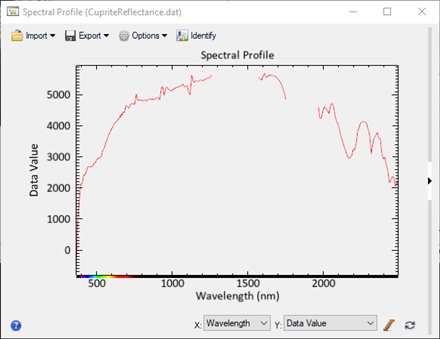
Gaps in the curve correspond to the bands that you just removed. Out of the original 224 AVIRIS bands, you are now working with 170. This is still sufficient for hyperspectral image analysis and material identification. See the Basic Hyperspectral Analysis tutorial to learn more about these concepts.
QUAC and FLAASH are registered trademarks of Spectral Sciences, Inc.