Basic feature extraction with ENVI ROIs
Anonym
The ENVI feature extraction module allows a user to extract certain features from an image. The first step is to segment the image in to regions. Once this is done, you can use spatial and spectral qualities of the regions to pull out targets.
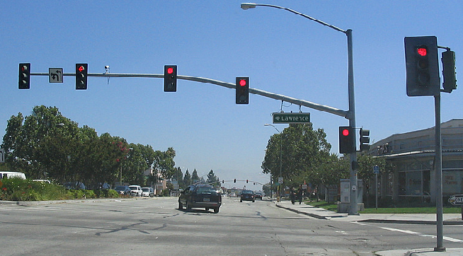
For this example, let’s find the traffic lights in this image taken from Wikipedia’s page on “traffic light”. https://en.wikipedia.org/wiki/Traffic_light
The first step is to do the segmentation with ENVI’s FXSegmention task. I’ve set a merge value of 85 and a segment value of 95, which I determined to be good values for this dataset through manual inspection in ENVI.
Once these segments are created, they can be converted to ENVI ROIs. In this case, I used the ImageThresholdToROI task.
From here, now we can look at qualities of each region, and create a scoring algorithm for how likely each ROI is the feature we are looking for. I felt like looking for the color red was not viable, as then this algorithm breaks down when the light changes. So instead, because our target regions we want to find are circular, let’s look for that.
There are two things we know about circles that we can check for. We know that they are symmetrical, and we know the relationship of the area and circumference as the radius of the circle increases. To start, I’ve set up the pixel coordinates of each ROI so that the origin is the average x/y location for that region. I’ve also calculated the distance away from the origin at each pixel.
x_avg = total(addr[0,*])/n_pix
y_avg = total(addr[1,*])/n_pix
x_coords = reform(addr[0,*] - x_avg)
y_coords = reform(addr[1,*] - y_avg)
power = (x_coords^2 +y_coords^2)
To test for symmetry, take the min and max of x and y, and add them together. The closer to zero that this value is, the more symmetric the ROI is.
abs(max(x_coords)+min(x_coords))+ abs(max(y_coords)+min(y_coords))
To test for how circular the area is, we can test the slope of how the distance from the origin increases. Since we know how this relationship between area and circumference behaves, we can find what slope we are looking for.
Slope =  = 1/3
= 1/3
Because a high score for symmetry is zero, let’s use the same scoring system for this measure.
line = linfit(lindgen(n_elements(power)),power[sort(power)])
score = abs(line[1]-.3333)
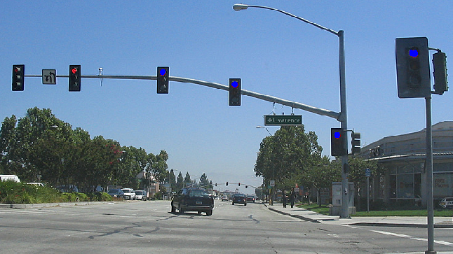
The final step is to assign weights (I used weights of 1) and calculate an overall score. The full code for extracting traffic lights (or any other circles) can be found at the bottom of this post.
This method for feature extraction takes a while to develop and perfect, which leads me to some exciting news for those that need to quickly develop feature extraction models. There is another method that we have been developing here in house to do feature extraction called MEGA, which is available through our Custom Solutions Group. This is a machine learning tool that takes in examples of a feature you are looking for, and then generates a heat map of where is it likely that that feature is located in an image.
Stay tuned for an in depth look at how this new method compares to classic feature extraction techniques like the one I’ve presented above.
pro traffic_light_fx
compile_opt idl2
file = 'C:\Blogs\FX_to_ROIs\Stevens_Creek_Blvd_traffic_light.jpg'
e=envi()
view = e.GetView()
;File was created from FX segmentation only. High Edge and Merge settings.
t0 = ENVITask('FXSegmentation')
raster = e.Openraster(file)
t0.INPUT_RASTER = raster
layer = view.CreateLayer(raster)
t0.OUTPUT_RASTER_URI = e.GetTemporaryFilename('.dat')
t0.MERGE_VALUE = 85.0
t0.SEGMENT_VALUE = 90.0
t0.Execute
t1 = envitask('ImageThresholdToROI')
t1.INPUT_RASTER = t0.OUTPUT_RASTER
t1.OUTPUT_ROI_URI = e.GetTemporaryFilename('.xml')
loop_max = max((t0.OUTPUT_RASTER).GetData(), MIN=loop_min)
num_areas = loop_max-loop_min+1
t1.ROI_NAME = 'FX_Area_' + strtrim(indgen(num_areas)+1, 2)
t1.ROI_COLOR = transpose([[bytarr(num_areas)],[bytarr(num_areas)],[bytarr(num_areas)+255]])
arr = indgen(num_areas) + loop_min
t1.THRESHOLD = transpose([[arr],[arr],[intarr(num_areas)]])
t1.execute
allROIs = t1.OUTPUT_ROI
c_scores = []
c_loc = []
for i=0, n_elements(allROIs)-1 do begin
addr = (allROIs[i]).PixelAddresses(raster)
n_pix = n_elements(addr)/2
if n_pix gt 60 then begin
x_avg = total(addr[0,*])/n_pix
y_avg = total(addr[1,*])/n_pix
x_coords = reform(addr[0,*] - x_avg)
y_coords = reform(addr[1,*] - y_avg)
power = (x_coords^2 + y_coords^2)
line = linfit(lindgen(n_elements(power)),power[sort(power)])
this_score = abs(max(x_coords) + min(x_coords)) + max(y_coords) + min(y_coords)) + abs(line[1]-.3333)
c_scores = [c_scores, this_score]
c_loc = [c_loc, i]
endif
endfor
idx = sort(c_scores)
sort_scores = c_scores[idx]
sort_locs = c_loc[idx]
for i=0, 3 do begin
lightROI = allROIs[sort_locs[i]]
!null = layer.AddRoi(lightROI)
endfor
end