Putting a Mountain Of Data In Your Hands - From a Point Cloud to a 3D Printed Model using ENVI LiDAR and IDL
For some of us, it's significantly easier to understand an object in 3-dimensional space if we're holding it in our hands, versus viewing it on a screen or even in a virtual reality environment.
Land-use or military planners, architects, and civil engineers will sometimes rely on scale models of their environment to better understand features of the terrain and the ramifications of their decisions.
This blog will cover one technique, using ENVI LiDAR along with some custom IDL code, to convert publicly-available LiDAR data into a 3-D printed object, a scale model.
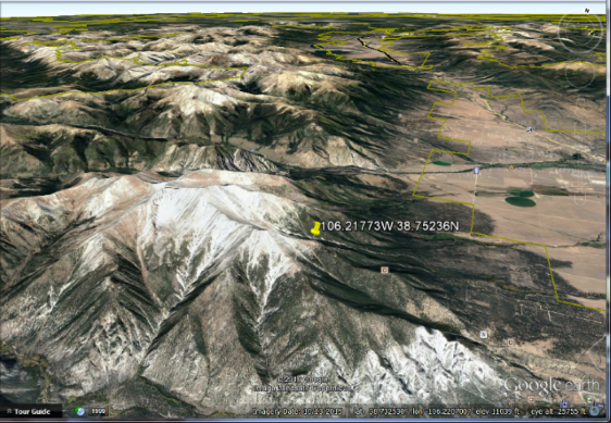
The subject of this study is a section of picturesque Mt. Princeton, a 14,196-foot peak that flanks the west side of the Arkansas River Valley near the town of Buena Vista, Colorado. Below is a Google Earth view of the region, for perspective.
LiDAR data for a section of the mountain is available to the public through the US Geological Survey's EarthExplorer online portal. Setting up a free account is simple.
Once online, navigate with the map display to the location of interest.
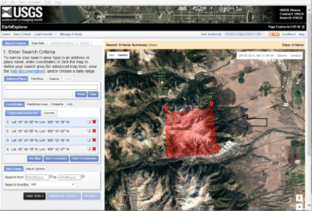
The initial goal is to determine which data sets are available for an area around the summit of Mt. Princeton. In this example, I have manually drawn a bounding box shown in red. Clicking the "Data Sets" button will bring you to the next page from which you can choose from among many data sources.
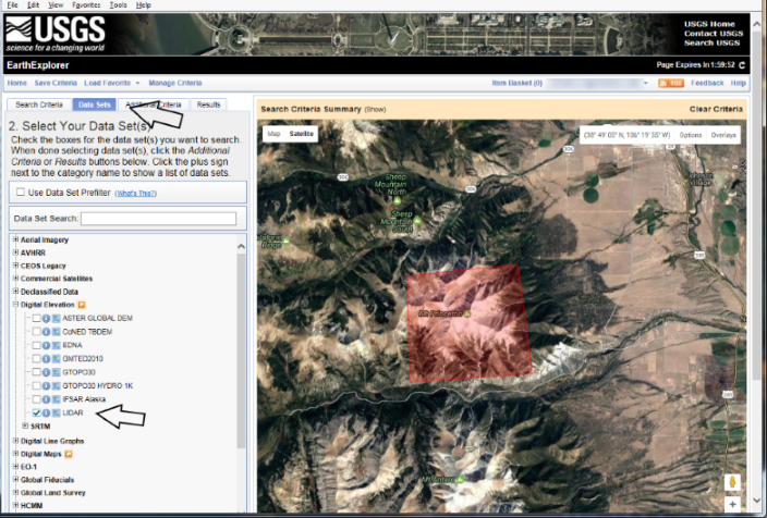
In order to generate a printed surface, we will start with the point cloud data associated with a LiDAR collection. Check the inventory of available data in this region of interest.
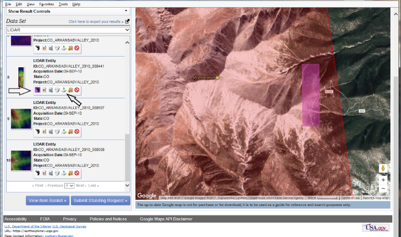
For each data set, the footprint icon will highlight the ground projection of the associated data in the image display. In this example, I've selected data set number 8, which shows fairly significant variations in elevation.
Clicking the "download" button for a data set will prompt you with a dialog box to choose the format of the output data.
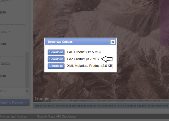
ENVI LiDAR can read compressed data as well as uncompressed data file formats, so I've selected the "LAZ Product" (compressed LiDAR) option to speed the transfer.
Download the resulting file to your local computer. Run ENVI 5.4 and select the downloaded ".laz" file as your input. You will be prompted initially for a coordinate system for the point cloud data because the map projection metadata is not carried with the point cloud in this format.
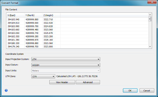
I know that this data set was collected in WGS84 in UTM zone 13 N coordinates. In reality, for our purposes of printing the data, the coordinate system is not particularly important. Unless you own a printer with an impressively large volume, we will be scaling and re-centering the units in the end, from meters to the scale of a few centimeters.
The original data in this area is approximately 1500 by 400 meters on the ground, with an altitude range of 500 meters.
When the projection is applied, the point data will be displayed in the ENVI LiDAR UI. Initially, this will include points returned from objects such as trees, rocks, hikers and marmots.
Point clouds cannot be printed directly because points do not occupy a physical volume. In this example, we will first create a polygonal mesh that represents a surface. The surface itself is not sufficient for 3-D printing, either, because a surface has no physical depth. But we will a third dimension in a future step.
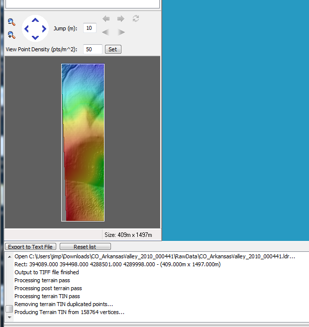
In order to create the initial surface model, we will use the Process Data option in ENVI LiDAR.
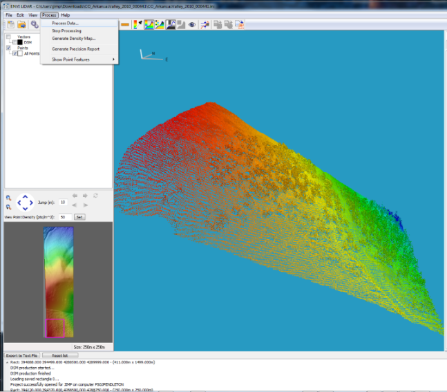
In this example, we will create a terrain surface model in the form of a Triangulated Irregular Network, or TIN. The TIN will provide the vertices and connectivity we need for printing the top of our physical object.
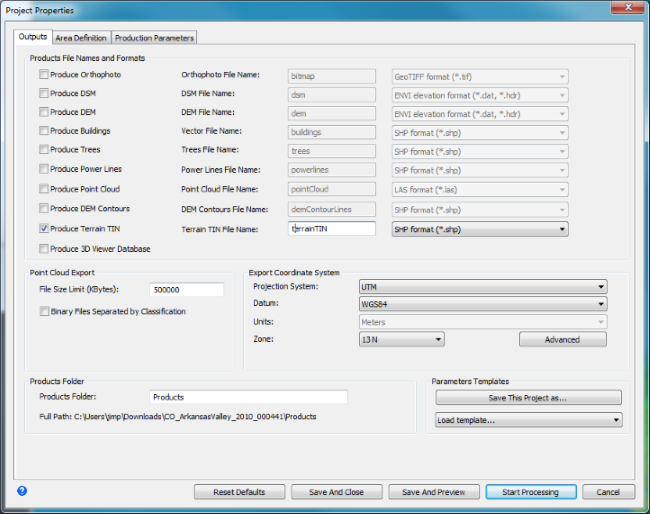
The vertices and connectivity will be written to a ShapeFile-format set of files, by default. Progress during processing is shown in the log window of ENVI LiDAR.
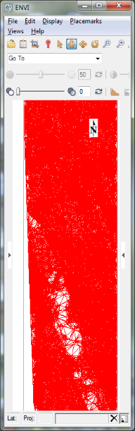
Close the ENVI LiDAR UI and return to the main ENVI UI. Select the ShapeFile you just created and display it.
From within ENVI, this View can be exported to Google Earth as an image that can be draped over the surface. Here is an associated tour.
In order to feed this surface model into a printer, we must first extract the data from the ShapeFile. The ShapeFile, as produced by ENVI LiDAR only stores the triangulation as one individual entity per triangle. As a result, there is a significant amount of duplication where multiple triangles will share a single vertex. In a later step, we will need to take into account this shared connectivity when locating the perimeter vertices.
The following IDL routine accepts as input the path to the .shp file and produces as output the vertex list and connectivity, removing duplicate vertices. Feel free to improve its efficiency.
pro shptopoly, file, v, c os = idlffshape(file) os.getproperty, n_entities = nen c = ulonarr(nen*4) tol = .005^2 ent = os.getentity(0) vc = *ent.vertices c[0] = [3L, 0, 1, 2] xs = reform(vc[0, 0:2]) ys = reform(vc[1, 0:2]) zs = reform(vc[2, 0:2]) vcount = 3LL for x = 1l, nen - 1 do begin ent = os.getentity(x) vc = *ent.vertices c[x*4] = 3 for i = 0l, 2 do begin r2 = min((vc[0, i] - xs)^2 + (vc[1, i] - ys)^2 + (vc[2, i] - zs)^2, mr2) if (r2 gt tol) then begin c[x*4 + i + 1] = vcount xs = [xs, reform(vc[0, i])] ys = [ys, reform(vc[1, i])] zs = [zs, reform(vc[2, i])] vcount++ endif else begin c[x*4 + i + 1] = mr2 endelse endfor endfor v = transpose([[xs], [ys], [zs]]) end
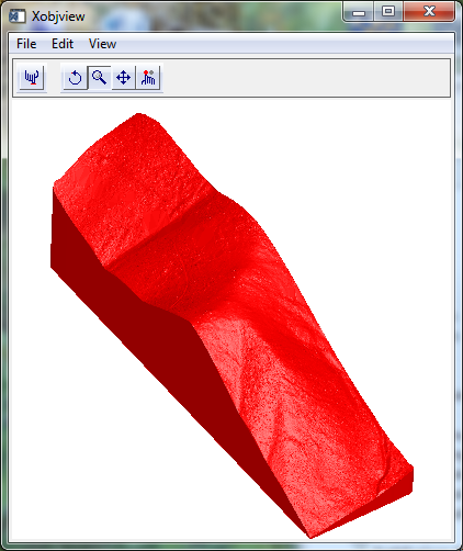
We can use this routine to compare our new model with the region of interest in EarthExplorer.
IDL> shptopoly, pathto + 'terrainTIN.shp', v, c
IDL> xobjview, idlgrpolygon(v, poly = c, color = !color.gold, style = 2)
Because a surface, by itself, has no depth it cannot be printed. One approach to adding depth is to create a "skirt" around the perimeter. First, we must locate the exterior vertices. An exterior vertex is one whose connected triangles fail to add to 360 degrees.
The following routine returns the indices of the exterior vertices. Feel free to optimize this routine as well.
function exteriorvertices, v, c compile_opt strictarr on_error, 2 indices = [] c0 = c[1:*:4] c1 = c[2:*:4] c2 = c[3:*:4] tol = 10./180*!dpi twopi = !dpi*2. for i = 0L, v.length/3 - 1 do begin hasvertex = where(c0 eq i or c1 eq i or c2 eq i, n) if (n eq 0) then continue allthetas = 0.d for j = 0L, n - 1 do begin v0 = double((v[*, c0[hasvertex[j]]])[0:1]) v1 = double((v[*, c1[hasvertex[j]]])[0:1]) v2 = double((v[*, c2[hasvertex[j]]])[0:1]) h = hasvertex[j] case 1 of c0[hasvertex[j]] eq i : begin aa = sqrt(total((v2 - v1)^2)) bb = sqrt(total((v0 - v1)^2)) cc = sqrt(total((v2 - v0)^2)) end c1[hasvertex[j]] eq i : begin aa = sqrt(total((v2 - v0)^2)) bb = sqrt(total((v1 - v0)^2)) cc = sqrt(total((v2 - v1)^2)) end c2[hasvertex[j]] eq i : begin aa = sqrt(total((v1 - v0)^2)) bb = sqrt(total((v2 - v1)^2)) cc = sqrt(total((v2 - v0)^2)) end else : endcase theta = acos((bb^2 + cc^2 - aa^2)/(2.*bb*cc)) allthetas += abs(theta) endfor if (abs(twopi - allthetas) gt tol) then indices = [indices, i] endfor return, indices end
Pass as input the vertices and connectivity list created earlier. The vector of indices is the function return value.
IDL> e = exteriorvertices(v, c)
(There are some edge cases not addressed in the code, such as edge triangles that are calculated by the TIN process to be perpendicular to the X-Y plane. How would you approach these?)
Given the exterior indices, we can now generate a polygonal mesh skirt for our model by projecting a new set of vertices "down" in the Z dimension to an arbitrary base depth that's lower than the lowest Z in the original data. Then we stitch the upper and lower exterior polygons with triangles to provide depth, and triangulate the base to fill it in as well.
pro addskirt, v, c, newv, newc, exterior_indices = e compile_opt strictarr newv = !null newc = !null newv = v mins = min(newv, dimension = 2, max = maxs) for i = 0, 1 do begin newv[i, *] -= mins[i] endfor if (e eq !null) then begin triangulate, newv[0, *], newv[1, *], tr, b endif else begin b = e endelse xmid= total(newv[0, b])/b.length ymid = total(newv[1, b])/b.length xx = newv[0, b] - xmid yy = newv[1, b] - ymid theta = atan(yy, xx) s = sort(theta) b = b[s] plots, newv[0, [b, b[0]]], newv[1, [b, b[0]]] oldx = reform(v[0, *]) oldy = reform(v[1, *]) oldz = reform(v[2, *]) oldc = oldx.length newx = [oldx, oldx[[b, b[0]]]] newy = [oldy, oldy[[b, b[0]]]] newz = [oldz, replicate(mins[2] - (maxs[2] - mins[2])/100., b.length + 1)] b = [b, b[0]] newc = c for i = 0, b.length - 2 do begin newc = [newc, 3, oldc + i, oldc + i + 1, b[i]] newc = [newc, 3, oldc + i + 1, b[i + 1], b[i]] endfor t = idlgrtessellator() t.addpolygon, oldx[b], oldy[b] r = t.tessellate(basev, basep) for i = 0, basep.length/4 - 1 do begin newc = [newc, 3, oldc + basep[[i*4 + 1 + lindgen(3)]]] endfor newv = transpose([[newx], [newy], [newz]]) newc mod= newv.length/3 opoly = idlgrpolygon(newv, poly = newc, style = 1, color = !color.red) xobjview, opoly end
This routine accepts as input the original vertices and connectivity list, along with the exterior vertex indices, and creates a new set of vertices and connectivity.
IDL> addskirt, v, c, newv, newc, exterior_indices = e
For debugging purposes, this call also visualizes the result in IDL.
Now we have a set of vertices and a connectivity list that is acceptable to most printing devices. But we must create a file that contains these coordinates in a format that can be used by a printer, or an interface that converts the data into a format acceptable to a particular printer.
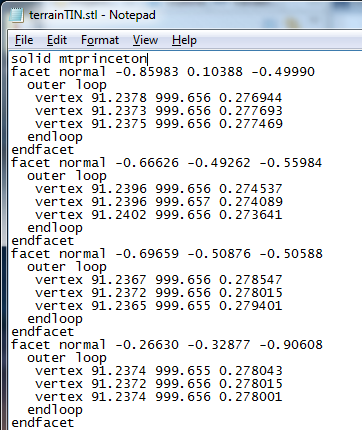
A very simple file format that is accepted by most printer drivers is STL, which is acronym-ish for "STereoLithography". In its simplest form, it is just a list of triangles.
The following code writes an ASCII-format STL file using our updated vertices and connectivity lists.
Pro MakeSTL, vertices, polygons, outfile On_Error, 2 Catch, ErrorNumber If (ErrorNumber ne 0) then Begin Catch, /Cancel If (LUN ne !null) then Begin Free_LUN, LUN EndIf If (C ne !null) then Begin CD, C Endif Message, /Reissue_Last Endif L = List() L.Add, 'solid mntprinceton' V = vertices For I = 0, 2 do begin V[I, *] -= min(Vertices[I, *]) EndFor Poly = Polygons For I = 0L, Poly.Length/4 - 1 Do Begin V1 = Reform(V[*, Poly[I*4 + 1]]) V2 = Reform(V[*, Poly[I*4 + 2]]) V3 = Reform(V[*, Poly[I*4 + 3]]) uu = v2 - v1 vv = v3 - v1 nx = uu[1]*vv[2] - uu[2]*vv[1] ny = uu[2]*vv[0] - uu[0]*vv[2] nz = uu[0]*vv[1] - uu[1]*vv[0] R = Sqrt(Total([nx,ny,nz]^2)) L.Add, 'facet normal ' + ((String([nx,ny,nz]/R, Format = '(f8.5)')).Trim()).Join(' ') L.Add, ' outer loop' L.Add, ' vertex ' + $ ((String(V1)).Trim()).Join(' ') L.Add, ' vertex ' + $ ((String(V2)).Trim()).Join(' ') L.Add, ' vertex ' + $ ((String(V3)).Trim()).Join(' ') L.Add, ' endloop' L.Add, 'endfacet' EndFor L.Add, 'endsolid mntprinceton' OpenW, LUN, OutFile, /Get_LUN ForEach Line, L Do Begin PrintF, LUN, Line EndForEach Free_LUN, LUN End
Call this routine with the new vertices and connectivity lists, along with a path to an output .stl file.
IDL> makestl, newv, newc, "path-to-your-output-file.stl"
The output file will be simple ASCII, with contents that resemble the following.
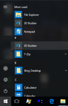
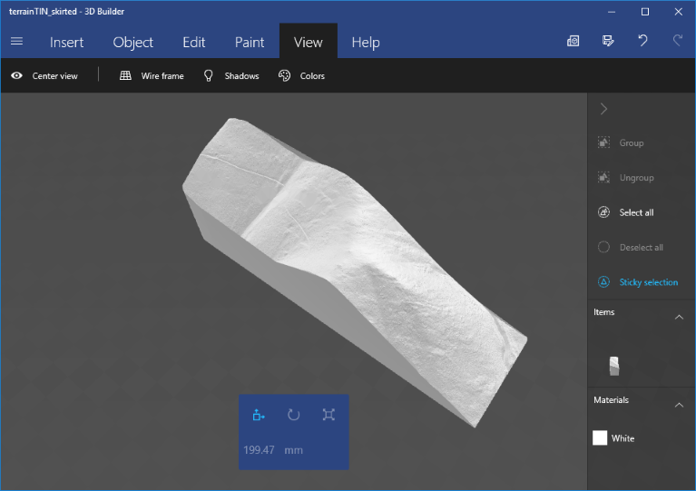
One option for printing the STL files is via the "3D Builder" application, which is available as a freebie in Windows 10.
Select the STL file as input. This will import the model into the printer driver, which is responsible for centering and scaling the raw data into the printer space.
Now you can print your data, if you have a printer. The 3D Builder application also has a convenient, if rather pricey, option to export your model to a third-party online service that will print your model remotely and ship it to you.
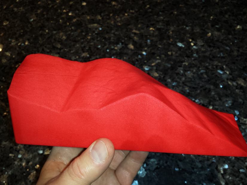
Here is the final product. Notice that the thin hiking trail is clearly visible.
If you have a more complicated model in ENVI or IDL and you would like some assistance generating a solid rendition, beyond what has been covered here, please contact NV5 Geospatial's Custom Solutions Group. We'd be happy to help!