WTN

The WTN function returns a multi-dimensional discrete wavelet transform of the input array A. The transform is based on a Daubechies wavelet filter.

WTN is based on the routine wtn described in section 13.10 of Numerical Recipes in C: The Art of Scientific Computing (Second Edition), published by Cambridge University Press, and is used by permission.

Syntax

Result = WTN( A, Coef [, /COLUMN] [, /DOUBLE] [, /INVERSE] [, /OVERWRITE] )

Return Value

Returns an output array of the same dimensions as A, containing the discrete wavelet transform over each dimension.

Arguments

A

The input vector or array. The dimensions of A must all be powers of 2.

Note: If WTN is complex then only the real part is used for the computation.

Coef

An integer that specifies the number of wavelet filter coefficients. The allowed values are 4, 12, or 20. When Coef is 4, the daub4() function (see Numerical Recipes, section 13.10) is used. When Coef is 12 or 20, pwt() is called, preceded by pwtset() (see Numerical Recipes, section 13.10).

Keywords

COLUMN

Set this keyword if the input array A is in column-major format (composed of column vectors) rather than in row-major format (composed of row vectors).

DOUBLE

Set this keyword to force the computation to be done in double-precision arithmetic.

INVERSE

If the INVERSE keyword is set, the inverse transform is computed. By default, WTN performs the forward wavelet transform.

OVERWRITE

Set the OVERWRITE keyword to perform the transform “in place.” The result overwrites the original contents of the array.

Examples

This example demonstrates the use of IDL’s discrete wavelet transform and sparse array storage format to compress and store an 8-bit gray-scale digital image. First, an image selected from the people.dat data file is transformed into its wavelet representation and written to a separate data file using the WRITEU procedure.

If you are viewing this topic from within the IDL Workbench, you can click on each code block in turn to execute the example.

; Begin by choosing the number of wavelet coefficients to use and a
; threshold value:
coeffs = 12 & thres = 10.0
; Open the people.dat data file, read an image using associated
; variables, and close the file:
OPENR, 1, FILEPATH('people.dat', SUBDIR = ['examples','data'])
images = ASSOC(1, BYTARR(192, 192, /NOZERO))
image_1 = images[0]
CLOSE, 1
; Expand the image to the nearest power of two using cubic
; convolution, and transform the image into its wavelet
; representation using the WTN function:
pwr = 256
image_1 = CONGRID(image_1, pwr, pwr, /CUBIC)
wtn_image = WTN(image_1, coeffs)
; Write the image to a file using the WRITEU procedure and check
; the size of the file (in bytes) using the FSTAT function:
OPENW, 1, 'original.dat'
WRITEU, 1, wtn_image
status = FSTAT(1)
CLOSE, 1
PRINT, 'Size of the file is ', status.size, ' bytes.'

Next, the transformed image is converted, using the SPRSIN function, to row-indexed sparse storage format retaining only elements with an absolute magnitude greater than or equal to a specified threshold. The sparse image is written to a data file using the WRITE_SPR procedure.

; Now, we convert the wavelet representation of the image to a
; row-indexed sparse storage format using the SPRSIN function,
; write the data to a file using the WRITE_SPR procedure, and check
; the size of the "compressed" file:
sprs_image = SPRSIN(wtn_image, THRES = thres)
WRITE_SPR, sprs_image, 'sparse.dat'
OPENR, 1, 'sparse.dat'
status = FSTAT(1)
CLOSE, 1
PRINT, 'Size of the compressed file is ', status.size, ' bytes.'
; Determine the number of elements (as a percentage of total
; elements) whose absolute magnitude is less than the specified
; threshold. These elements are not retained in the row-indexed
; sparse storage format:
PRINT, 'Percentage of elements under threshold: ',$
   100.*N_ELEMENTS(WHERE(ABS(wtn_image) LT thres, $
   count)) / N_ELEMENTS(image_1)

Finally, the transformed image is reconstructed from the storage file and displayed alongside the original.

; Next, read the row-indexed sparse data back from the file
; sparse.dat using the READ_SPR function and reconstruct the
; image from the non-zero data using the FULSTR function:
sprs_image = READ_SPR('sparse.dat')
wtn_image = FULSTR(sprs_image)
; Apply the inverse wavelet transform to the image:
image_2 = WTN(wtn_image, COEFFS, /INVERSE)
; Finally, display the original and reconstructed 
; images side by side:
WINDOW, 1, XSIZE = pwr*2, YSIZE = pwr, $
   TITLE = 'Wavelet Image Compression and File I/O'
TV, image_1, 0, 0
TV, image_2, pwr - 1, 0
; Calculate and print the amount of data used in

; reconstruction of the image:
PRINT, 'The image on the right is reconstructed from:', $
   100.0 - (100.* count/N_ELEMENTS(image_1)),$
   '% of original image data.'

IDL Output

Size of the file is   262144 bytes.

Size of the compressed file is   69600 bytes.

Percentage of elements under threshold:   87.0331

The image on the right is reconstructed from: 12.9669% of original image data.

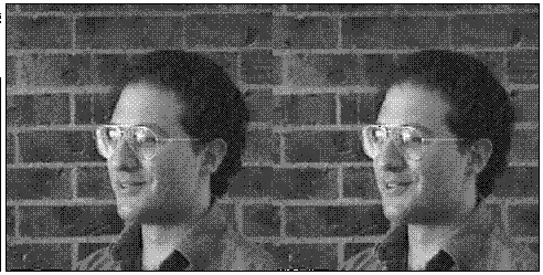
The sparse array contains only 13% of the elements contained in the original array. The following figure is created from this example. The image on the left is the original 256 by 256 image. The image on the right was compressed by the above process and was reconstructed from 13% of the original data. The size of the compressed image’s data file is 26.6% of the size of the original image’s data file. Note that due to limitations in the printing process, differences between the images may not be as evident as they would be on a high-resolution printer or monitor. The following shows the original image (left) and image reconstructed from 13% of the data (right).

Version History

4.0	Introduced

WTN