DERIV

The DERIV function uses three-point (quadratic) Lagrangian interpolation to compute the derivative of an evenly-spaced or unevenly-spaced array of data.

Given three neighboring points in your data with X coordinates [x₀, x₁, x₂] and Y coordinates [y₀, y₁, y₂], the three-point Lagrangian interpolation polynomial is defined as:

y = y₀(x – x₁)(x – x₂)/[(x₀ – x₁)(x₀ – x₂)] +

y₁(x – x₀)(x – x₂)/[(x₁ – x₀)(x₁ – x₂)] +

y₂(x – x₀)(x – x₁)/[(x₂ – x₀)(x₂ – x₁)]

This can be rewritten as:

y = y₀(x – x₁)(x – x₂)/(x₀₁x₀₂) – y₁(x – x₀)(x – x₂)/(x₀₁x₁₂) + y₂(x – x₀)(x – x₁)/(x₀₂x₁₂)

where x₀₁ = x₀ – x₁, x₀₂ = x₀ – x₂, and x₁₂ = x₁ – x₂.

Taking the derivative with respect to x:

y' = y₀(2x – x₁ – x₂)/(x₀₁x₀₂) – y₁(2x – x₀ – x₂)/(x₀₁x₁₂) + y₂(2x – x₀ – x₁)/(x₀₂x₁₂)

Given a discrete set of X locations and Y values, the DERIV function then computes the derivative at all of the X locations. For example, for all of the X locations (except the first and last points), the derivative y' is computed by substituting in x = x₁:

y' = y₀x₁₂/(x₀₁x₀₂) + y₁(1/x₁₂ – 1/x₀₁) – y₂x₀₁/(x₀₂x₁₂)

The first point is computed at x = x₀:

y' = y₀(x₀₁ + x₀₂)/(x₀₁x₀₂) – y₁x₀₂/(x₀₁x₁₂) + y₂x₀₁/(x₀₂x₁₂)

The last point is computed at x = x₂:

y' = –y₀x₁₂/(x₀₁x₀₂) + y₁x₀₂/(x₀₁x₁₂) – y₂(x₀₂ + x₁₂)/(x₀₂x₁₂)

For an evenly-spaced array of values Y[0...N–1], the three-point Lagrangian interpolation reduces to:

Y'[0] = (–3*Y[0] + 4*Y[1] – Y[2]) / 2

Y'[i] = (Y[i+1] – Y[i–1]) / 2 ; i = 1...N–2

Y'[N–1] = (3*Y[N–1] – 4*Y[N–2] + Y[N–3]) / 2

This routine is written in the IDL language. You can find more details for all of the above equations in the source code in the file deriv.pro in the lib subdirectory of the IDL distribution.

Example

Compute the derivative of the sin function:

x = [0:10:0.01]

y = sin(x)

dy = DERIV(x, y)

help, dy

print, max(abs(dy - cos(x)))

IDL prints:

DY              FLOAT     = Array[1001]

3.33786e-005

Syntax

Result = DERIV([X,] Y)

Return Value

Returns a one-dimensional array of values containing the derivative of Y. If either X or Y is double precision then the result will be double precision, otherwise the result will be single precision.

Arguments

X

A one-dimensional array of data containing the X locations. If X is omitted then the Y points are assumed to be evenly spaced.

Y

A one-dimensional array of data containing the Y values.

Version History

Pre 4.0	Introduced
8.3	Add theory and examples

Another Example

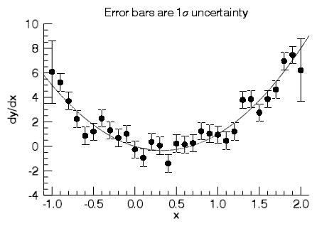Here, we compute the derivative of the function x³ – x² + 1 with some added Gaussian random noise. We then use DERIVSIG to compute the error estimates. Finally, we make an errorbar plot of the derivative and overplot the theoretical derivative 3x² – 2x.

x = [-1:2:0.1]

y = x^3 - x^2 + 1 + 0.1*randomn(2,n_elements(x))

dy = DERIV(x, y)

sigd = DERIVSIG(x, y, 0, 0.1)

p = ERRORPLOT(x, dy, sigd, 'o', /SYM_FILLED, $

  AXIS_STYLE=1, DIM=[300,300], $

  XRANGE=[-1.1,2.1], $

  XTITLE='x', YTITLE='dy/dx', $

  TITLE='Error bars are 1$\sigma$ uncertainty')

p = PLOT('3*x^2 - 2*x', /OVERPLOT)

print, CORRELATE(dy, 3*x^2 - 2*x)

IDL prints:

0.940621

Resources and References

F. B. Hildebrand, Introduction to Numerical Analysis, 2nd ed., Dover Books, 1987, p. 85.

P.R. Bevington and D. K. Robinson, Data Analysis and Reduction for the Physical Sciences, 3rd ed., McGraw-Hill, 2002, p. 39.