The FFT function returns a result equal to the complex, discrete Fourier transform of Array. The result of this function is a single- or double-precision complex array.
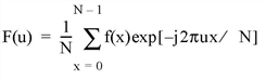
The discrete Fourier transform, F(u), of an N-element, one-dimensional function, f(x), is defined as:
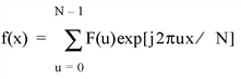
And the inverse transform, (Direction > 0), is defined as:
If the keyword OVERWRITE is set, the transform is performed in-place, and the result overwrites the original contents of the array.
See Fast Fourier Transform Background for more information on how FFT is used to reduce background noise in imagery.
Example
The following code plots the logarithm of the power spectrum of a 100-element index array:
p = PLOT(ABS(FFT(FINDGEN(100), -1)), /YLOG)
Additional Examples
See Additional Examples and Fast Fourier Transform for more code examples using the FFT function.
Algorithm & Running Time
FFT uses a multivariate complex Fourier transform, computed in place with a mixed-radix Fast Fourier Transform algorithm.
The FFT algorithm is implemented differently based on platform and the number of dimensions:
-
Intel x86_64 (Linux, Mac, Windows): For all arrays less than 8 dimensions, FFT calls the Intel Math Kernel Library Fast Fourier Transform. For arrays of 8 dimensions, FFT uses Fortran code authored by RC Singleton (Stanford Research Institute, September 1968 (NIST Guide to Available Math Software) and translated by f2c (version 19950721; MJ Olesen, Queen's University at Kingston, 1995-97; retrieved from NETLIB January 2000).
-
Arm64 (Apple Silicon, M-series Macs): FFT calls the Arm Performance Libraries (ArmPL) FFT functions.
For a one-dimensional FFT, running time is roughly proportional to the total number of points in Array times the sum of its prime factors. Let N be the total number of elements in Array, and decompose N into its prime factors:
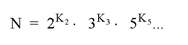
Running time is proportional to:
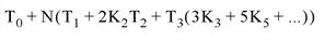
where T3 ~ 4T2. For example, the running time of a 263 point FFT is approximately 10 times longer than that of a 264 point FFT, even though there are fewer points. The sum of the prime factors of 263 is 264 (1 + 263), while the sum of the prime factors of 264 is 20 (2 + 2 + 2 + 3 + 11).
Syntax
Result = FFT( Array [, Direction] [, /CENTER] [, DIMENSION=scalar] [, /DOUBLE] [, /INVERSE] [, /OVERWRITE] )
Return Value
FFT returns a complex array that has the same dimensions as the input array. The output array is ordered in the same manner as almost all discrete Fourier transforms. Element 0 contains the zero frequency component, F0. The array element F1 contains the smallest, nonzero positive frequency, which is equal to 1/(Ni Ti), where Ni is the number of elements and Ti is the sampling interval of the ith dimension. F2 corresponds to a frequency of 2/(Ni Ti). Negative frequencies are stored in the reverse order of positive frequencies, ranging from the highest to lowest negative frequencies.
Note: The FFT function can be performed on functions of up to eight (8) dimensions. If a function has n dimensions, IDL performs a transform in each dimension separately, starting with the first dimension and progressing sequentially to dimension n. For example, if the function has two dimensions, IDL first does the FFT row by row, and then column by column.
For an even number of points in the ith dimension, the frequencies corresponding to the returned complex values are:
0, 1/(NiTi), 2/(NiTi), ..., (Ni/2–1)/(NiTi), 1/(2Ti), –(Ni/2–1)/(NiTi), ..., –1/(NiTi)
where 1/(2Ti) is the Nyquist critical frequency.
For an odd number of points in the ith dimension, the frequencies corresponding to the returned complex values are:
0, 1/(NiTi), 2/(NiTi), ..., (Ni–1)/2)/(NiTi), –(Ni–1)/2)/(NiTi), ..., –1/(NiTi)
In IDL code, these frequencies may be computed as follows:
X = FINDGEN((N - 1)/2) + 1
is_N_even = (N MOD 2) EQ 0
if (is_N_even) then $
freq = [0.0, X, N/2, -N/2 + X]/(N*T) $
else $
freq = [0.0, X, -(N/2 + 1) + X]/(N*T)
Arguments
Array
The array to which the Fast Fourier Transform should be applied. If Array is not of complex type, it is converted to complex type. The dimensions of the result are identical to those of Array. The size of each dimension may be any integer value and does not necessarily have to be an integer power of 2, although powers of 2 are certainly the most efficient.
Direction
Direction is a scalar indicating the direction of the transform, which is negative by convention for the forward transform, and positive for the inverse transform. If Direction is not specified, the forward transform is performed.
A normalization factor of 1/N, where N is the number of points, is applied during the forward transform.
Note: When transforming from a real vector to complex and back, it is slightly faster to set Direction to 1 in the real to complex FFT.
Note also that the value of Direction is ignored if the INVERSE keyword is set.
Keywords
CENTER
Set this keyword to shift the zero-frequency component to the center of the spectrum. In the forward direction, when CENTER is set, the resulting Fourier transform has the zero-frequency component shifted to the center of the array. In the reverse direction, when CENTER is set, the input is assumed to be a centered Fourier transform, and the coefficients are shifted back before performing the inverse transform.
Note: For an odd number of points the zero-frequency component will be in the center. For an even number of points the first element will correspond to the Nyquist frequency component, followed by the remaining frequency components - the zero-frequency component will then be in the center of the remaining components.
DIMENSION
Set this keyword to a scalar indicating the dimension across which to calculate the FFT. If this keyword is not present or is zero, then the FFT is computed across all dimensions of the input array. If this keyword is present, then the FFT is only calculated only across a single dimension. For example, if the dimensions of Array are N1, N2, N3, and DIMENSION is 2, the FFT is calculated only across the second dimension.
Note: If the CENTER keyword is also set, then only the dimension given by the DIMENSION keyword is shifted to the center. The other dimensions remain unshifted.
DOUBLE
Set this keyword to a value other than zero to force the computation to be done in double-precision arithmetic, and to give a result of double-precision complex type. If DOUBLE is set equal to zero, computation is done in single-precision arithmetic and the result is single-precision complex. If DOUBLE is not specified, the data type of the result will match the data type of Array.
INVERSE
Set this keyword to perform an inverse transform. Setting this keyword is equivalent to setting the Direction argument to a positive value. Note, however, that setting INVERSE results in an inverse transform even if Direction is specified as negative.
OVERWRITE
If this keyword is set, and the Array parameter is a variable of complex type, the transform is done “in-place”. The result overwrites the previous contents of the variable.
For example, to perform a forward, in-place FFT on the variable a:
a = FFT(a, -1, /OVERWRITE)
Thread Pool Keywords
On Intel x86_64 platforms, this routine is written to make use of IDL’s thread pool, which can increase execution speed on systems with multiple CPUs. The values stored in the !CPU system variable control whether IDL uses the thread pool for a given computation. In addition, you can use the thread pool keywords TPOOL_MAX_ELTS, TPOOL_MIN_ELTS, and TPOOL_NOTHREAD to override the defaults established by !CPU for a single invocation of this routine. See Thread Pool Keywords for details.
On the arm64, M-series Mac platform the IDL thread pool settings and keywords are ignored.
Note: Specifically, FFT will use the thread pool to overlap the inner loops of the computation when used on data with dimensions which have factors of 2, 3, 4, or 5. The prime-number DFT does not use the thread pool, as doing so would yield a relatively small benefit for the complexity it would introduce. Our experience shows that the improvement in performance from using the thread pool for FFT is highly dependent upon many factors (data length and dimensions, single vs. double precision, operating system, and hardware) and can vary between platforms.
Additional Examples
Example 1
In this example we display the power spectrum of a 100-element vector sampled at a rate of 0.1 seconds per point. The 0 frequency component is displayed at the center of the plot, and frequency is plotted on the x-axis:
N = 100
T = 0.1
N21 = N/2 + 1
F = INDGEN(N)
F[N21] = N21 -N + FINDGEN(N21-2)
F = F/(N*T)
p = PLOT(SHIFT(F, -N21), SHIFT(ABS(FFT(F, -1)), -N21), /YLOG)
Example 2
In this example we compute the FFT of two-dimensional images:
n = 256
x = FINDGEN(n)
y = COS(x*!PI/6)*EXP(-((x - n/2)/30)^2/2)
z = REBIN(y, n, n)
z = ROT(z, 10) + ROT(z, -45)
LOADCT, 39
p = IMAGE(BYTSCL(z), LAYOUT = [2, 2, 1])
f = FFT(z)
logpower = ALOG10(ABS(f)^2)
p = IMAGE(BYTSCL(logpower), LAYOUT = [2, 2, 2], /CURRENT)
f = FFT(z, DIMENSION=1)
logpower = ALOG10(ABS(f)^2)
p = IMAGE(BYTSCL(logpower), LAYOUT = [2, 2, 3], /CURRENT)
f = FFT(z, DIMENSION=2)
logpower = ALOG10(ABS(f)^2)
p = IMAGE(BYTSCL(logpower), LAYOUT = [2, 2, 4], /CURRENT)
Version History
|
Original |
Introduced |
|
7.1 |
Added CENTER keyword
|
| 8.4.1 |
Bug fix: When both DIMENSION and CENTER are set, only DIMENSION is shifted to the center; all other dimensions remain unshifted. |
| 8.8.1 |
Changed algorithm to use Intel Math Kernel Library Fast Fourier Transform |
| 9.0 |
Implemented algorithm on arm64 Mac to use the Arm Performance Libraries (ArmPL) |
See Also
FFT_POWERSPECTRUM, HILBERT