BANDPASS_FILTER

The BANDPASS_FILTER function applies a lowpass, bandpass, or highpass filter to a one-channel image.

A bandpass filter is useful when the general location of the noise in the frequency domain is known. The bandpass filter allows frequencies within the chosen range through and attenuates frequencies outside of the given range.

The following diagrams give a visual interpretation of the transfer functions:

This routine is written in the IDL language. Its source code can be found in the file bandpass_filter.pro in the lib subdirectory of the IDL distribution.

Syntax

Result = BANDPASS_FILTER( ImageData, LowFreq, HighFreq [, /IDEAL] [, BUTTERWORTH=value] [, /GAUSSIAN] )

Return Value

Returns a filtered image array of the same dimensions and type as ImageData.

Arguments

ImageData

A two-dimensional array containing the pixel values of the input image.

LowFreq

The lower limit of the pass-through frequency band. This value should be between 0 and 1 (inclusive), and must be less than HighFreq.

HighFreq

The upper limit of the pass-through frequency band. This value should be between 0 and 1 (inclusive), and must be greater than LowFreq.

Keywords

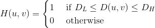
IDEAL

Set this keyword to use an ideal bandpass filter. In ideal bandpass filters, frequencies within the given range are passed through without attenuation and frequencies outside of the given range are completely removed. This behavior makes ideal bandpass filters very sharp.

The centered Fast Fourier Transform (FFT) is filtered by the following function, where D_L is the lower bound of the frequency band, D_H is the upper bound of the frequency band, and D(u,v) is the distance between a point (u,v) in the frequency domain and the center of the frequency rectangle:

BUTTERWORTH

Set this keyword to the dimension of the Butterworth filter to apply to the frequency domain. With a Butterworth bandpass filter, frequencies at the center of the frequency band are unattenuated and frequencies at the edge of the band are attenuated by a fraction of the maximum value. The Butterworth filter does not have sharp discontinuities between frequencies that are passed and filtered.

The default for BANDPASS_FILTER is BUTTERWORTH=1.

The centered FFT is filtered by one of the following functions, where D₀ is the center of the frequency band, W is the width of the frequency band, D=D(u,v) is the distance between a point (u,v) in the frequency domain and the center of the frequency rectangle, and n is the dimension of the Butterworth filter:

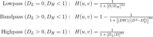
A low Butterworth dimension is close to Gaussian, and a high Butterworth dimension is close to Ideal.

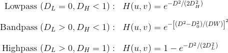
GAUSSIAN

Set this keyword to use a Gaussian bandpass filter. In this type of filter, the transition between unfiltered and filtered frequencies is very smooth.

The centered FFT is filtered by one of the following functions, where D₀ is the center of the frequency band, W is the width of the frequency band, and D=D(u,v) is the distance between a point (u,v) in the frequency domain and the center of the frequency rectangle:

Examples

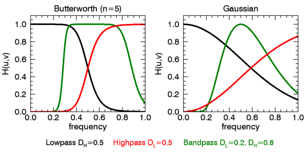
Here, we plot the frequency response of the Butterworth (n=5) and Gaussian filters. For the lowpass filter we use a high-frequency cutoff of 0.5, for highpass we use a cutoff of 0.5, and for the bandpass we use D_L=0.2 and D_H=0.8.

m = [0.2,0.27,0.05,0.1]

p = PLOT('1/(1 + (X/0.5)^10)', '3', DIM=[600,300], FONT_SIZE=10, $

  XRANGE=[0,1], YRANGE=[0,1.1], LAYOUT=[2,1,1], MARGIN=m, $

  XTITLE='frequency', YTITLE='H(u,v)', TITLE='Butterworth (n=5)')

p = PLOT('1-1/(1 + (X*0.6/(X^2-0.5^2))^10)', '3g', /OVERPLOT)

p = PLOT('1/(1 + (0.5/X)^10)', '3r', /OVERPLOT)

p = PLOT('exp(-X^2/(2*0.5^2))', '3', DIM=[600,300], FONT_SIZE=10, $

  XRANGE=[0,1], YRANGE=[0,1.1], LAYOUT=[2,1,2], MARGIN=m, $

  XTITLE='frequency', YTITLE='H(u,v)', TITLE='Gaussian', /CURRENT)

p = PLOT('exp(-((X^2-0.5^2)/(X*0.6))^2)', '3g', /OVERPLOT)

p = PLOT('1-exp(-X^2/(2*0.5^2))', '3r', /OVERPLOT)

t = TEXT(0.15,0.05,'Lowpass $D_H=0.5$',/NORM, FONT_SIZE=9)

t = TEXT(0.37,0.05,'Highpass $D_L=0.5$',COLOR='red',/NORM, FONT_SIZE=9)

t = TEXT(0.6,0.05,'Bandpass $D_L=0.2, D_H=0.8$',COLOR='green',/NORM, FONT_SIZE=9)

p.Save, 'bandpass_filter.png', resolution=120

In the following example, we add some sinusoidal noise to an image and filter it with BANDPASS_FILTER, using the BUTTERWORTH keyword.

; Read in the file

file = FILEPATH('moon_landing.png', SUBDIR=['examples','data'])

imageOriginal = READ_PNG(file)

; Generate some sinusoidal noise

xCoords = LINDGEN(300,300) MOD 300

yCoords = TRANSPOSE(xCoords)

noise = -SIN(xCoords*2)-SIN(yCoords*2)

imageNoise = imageOriginal + 50*noise

; Filter using a lowpass filter

imageFiltered = BANDPASS_FILTER(imageNoise, 0, 0.4, $

  BUTTERWORTH=20)

; Display the original, noise-added, and filtered images

i=IMAGE(imageOriginal, LAYOUT=[3,1,1], TITLE='Original Image', $

  DIMENSIONS=[700,300])

i=IMAGE(imageNoise, LAYOUT=[3,1,2], /CURRENT, TITLE='Added Noise')

i=IMAGE(imageFiltered, LAYOUT=[3,1,3], /CURRENT, $

  TITLE='Butterworth Filtered')

i.Save, 'bandpass_filter_butterworth_ex.gif', resolution=120

Reference

Gonzalez, R.C., and R.E. Woods. Digital Image Processing, 3rd edition. Pearson Education, Upper Saddle River, New Jersey, 2008.

Version History

7.1	Introduced
8.5.2	Add equations for lowpass and highpass filters.