The KRIG2D function using the kriging method to interpolate a regularly- or irregularly-gridded set of points to a regular grid.
The parameters of the data model – the range, nugget, and sill – are highly dependent upon the degree and type of spatial variation of your data, and should be determined statistically. Experimentation, or preferably rigorous analysis, is required.
For n data points, a system of n+1 simultaneous equations are solved for the coefficients of the surface. For any output point, the interpolated value is then given by the sum of all of the input points, weighted by the distance of each input point to the desired output point. Four different models are available for the weighting function. The equations are shown in the plot below:
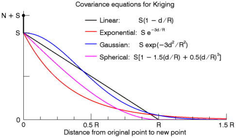
In the above equations, N is the Nugget value, S is the Scale, and R is the Range. The value d is the distance from a point in the input array to a point in the result. All four models have a covariance weighting of N + S at d=0. The Linear and Spherical models are both zero for d > R.
- At distances beyond R, the semivariogram or covariance remains essentially constant.
- The nugget N provides a discontinuity at the origin.
- The scale S is optional. If specified, S is the covariance value for a zero distance, and the variance of the random sample z variable. If only a two element vector is supplied for the model parameters, S is set to the sample variance.
This routine is written in the IDL language. Its source code can be found in the file krig2d.pro in the lib subdirectory of the IDL distribution.
Example
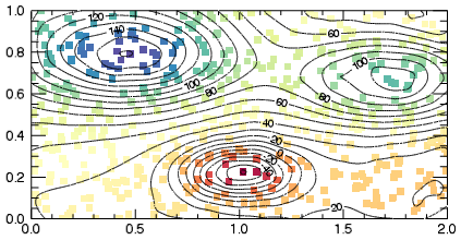
In the following example, we create an irregularly-gridded 2-D data set. The KRIG2D function interpolates the data at a specified grid size. The resulting plot is shown at the top of this topic.
n = 500
seed = -121147L
x = 2*RANDOMU(seed, n)
y = RANDOMU(seed, n)
z = 100*(EXP(-((4*x-2)^2 + (7-9*y)^2)/4) + $
EXP(-((4*x+1)^2)/49 - (1-0.9*y)) + $
EXP(-((4*x-7)^2 + (6-9*y)^2)/4) - $
EXP(-(4*x-4)^2 - (2-9*y)^2))
result = KRIG2D(z, x, y, EXPONENTIAL=[0.5,0.2,1], $
NX=200, NY=200, XOUT=xout, YOUT=yout)
p = PLOT(x, y, 's', RGB_TABLE=74, ASPECT_RATIO=1, $
/SYM_FILLED, VERT_COLORS=BYTSCL(z))
c = CONTOUR(result, xout, yout, C_THICK=2, $
COLOR='black', C_VALUE=[-60:160:10], /OVERPLOT)
Syntax
Result = KRIG2D( Z [, X, Y] [, /DOUBLE] [, EXPONENTIAL=vector] [, GAUSSIAN=vector] [, LINEAR=vector] [, SPHERICAL=vector] [, /REGULAR] [, XGRID=[xstart, xspacing]] [, XVALUES=array] [, YGRID=[ystart, yspacing]] [, YVALUES=array] [, GS=[xspacing, yspacing]] [, BOUNDS=[xmin, ymin, xmax, ymax]] [, NX=value] [, NY=value] [, XOUT=variable] [, YOUT=variable] )
Return Value
Returns a two dimensional floating-point array containing the interpolated surface, sampled at the grid points.
Arguments
Z, X, Y
Arrays containing the Z, X, and Y coordinates of the data points on the surface. Points need not be regularly gridded. For regularly gridded input data, X and Y are not used: the grid spacing is specified via the XGRID and YGRID (or XVALUES and YVALUES) keywords, and Z must be a two dimensional array. For irregular grids, all three parameters must be present and have the same number of elements.
Keywords
DOUBLE
Set this keyword to force the computation to be done using double-precision arithmetic, and return a double-precision result. By default, single precision is used, regardless of the precision of the input arrays.
XOUT
Set this keyword to a named variable in which to return a vector containing the output X coordinates.
YOUT
Set this keyword to a named variable in which to return a vector containing the output Y coordinates.
Model Parameter Keywords:
EXPONENTIAL
Set this keyword to a two- or three-element vector of model parameters [R, N] or [R, N, S] to use the exponential semivariogram model.
GAUSSIAN
Set this keyword to a two- or three-element vector of model parameters [R, N] or [R, N, S] to use the Gaussian semivariogram model.
LINEAR
Set this keyword to a two- or three-element vector of model parameters [R, N] or [R, N, S] to use the linear semivariogram model.
SPHERICAL
Set this keyword to a two- or three-element vector of model parameters [R, N] or [R, N, S] to use the spherical semivariogram model.
Input Grid Keywords:
REGULAR
If set, the Z parameter is a two dimensional array of dimensions (n,m), containing measurements over a regular grid. If any of XGRID, YGRID, XVALUES, or YVALUES are specified, REGULAR is implied. REGULAR is also implied if there is only one parameter, Z. If REGULAR is set, and no grid specifications are present, the grid is set to (0, 1, 2, ...).
XGRID
A two-element array, [xstart, xspacing], defining the input grid in the x direction. Do not specify both XGRID and XVALUES.
XVALUES
An n-element array defining the x locations of Z[i,j]. Do not specify both XGRID and XVALUES.
YGRID
A two-element array, [ystart, yspacing], defining the input grid in the y direction. Do not specify both YGRID and YVALUES.
YVALUES
An n-element array defining the y locations of Z[i,j]. Do not specify both YGRID and YVALUES.
Output Grid Keywords:
BOUNDS
If present, BOUNDS must be a four-element array containing the grid limits in x and y of the output grid: [xmin, ymin, xmax, ymax]. If not specified, the grid limits are set to the extent of x and y.
GS
The output grid spacing. If present, GS must be a two-element vector [xs, ys], where xs is the horizontal spacing between grid points and ys is the vertical spacing. The default is based on the extents of x and y. If the grid starts at x value xmin and ends at xmax, then the default horizontal spacing is (xmax - xmin)/(NX-1). ys is computed in the same way. The default grid size, if neither NX or NY are specified, is 26 by 26.
NX
The output grid size in the x direction. NX need not be specified if the size can be inferred from GS and BOUNDS. The default value is 26.
NY
The output grid size in the y direction. NY need not be specified if the size can be inferred from GS and BOUNDS. The default value is 26.
Version History
|
Pre 4.0 |
Introduced |
| 8.3 |
Added DOUBLE, GAUSSIAN, LINEAR, XOUT, and YOUT keywords. Rewrote the algorithm to improve performance. |
See Also
BILINEAR, GRIDDATA, INTERPOLATE