The IDL Machine Learning framework provides a powerful and flexible way to run machine learning applications on numerical data. You can create and train models and apply them in classification, clustering, or regression applications.
For a detailed example of how to use the IDL Machine Learning Framework to train a model that learns to recognize hand-written digits, compile and run classify_digits.pro, which is located in the examples/machine_learning directory of your IDL installation.
This topic provides basic concepts and workflows to get started with IDL Machine Learning. The following steps are described here.
- Prepare Data: How to get data ready to use in machine learning.
- Classification: Use examples to train a model that will predict a discrete output class (only a finite number of outputs is possible).
- Clustering: Use examples to train a model that will cluster a dataset into a given number of groups or clusters.
- Regression: Use examples to train a model that will predict a continuous output value (an infinite number of output values is possible).
Prepare Data
The first step in machine learning is to identify your input data. The input data is a set of numerical attributes that will feed your model to produce an output. There are two important considerations when preparing your data:
- Data normalization: Machine learning algorithms work best if the data is constrained to a [0 to 1] or [-1 to 1] range. Use a normalizer to perform this task, which is described in the examples that follow. The normalizers are: IDLmlLinearNormalizer, IDLmlRangeNormalizer, IDLmlTanHNormalizer, IDLmlUnitNormalizer, IDLmlVarianceNormalizer.
- Data separation: Prepare two groups of data. One group is used for training the model, the other is used to test its accuracy. It is recommended that you do not use the same data for training and testing. Depending on how you read your data, two helper routines can split the data: IDLmlShuffle and IDLmlPartition. Shuffling randomizes the order of the features and values. Partitioning separates the data into two or more groups, where each group contains a specific quantity of the elements.
To illustrate these steps, start by reading some data:
read_seeds_example_data, features, labels
This routine reads a CSV file that ships with IDL and returns two arrays: Features and Labels. Features is an array of 7 x 210 elements. Each column represents a different attribute (area, perimeter, compactness, length, width, asymmetry coefficient, and length of kernel groove), and there are 210 different instances. Labels is a string array of 210 elements that contain the type of seed (Kama, Rosa, or Canadian).
Below shows a preview of 13 rows (out of 210) of the CSV file:
|
Area |
Perimeter |
Compactness |
Length
of Kernel
|
Width
of Kernel
|
Asymmetry
Coefficient
|
Length of
Kernel Groove
|
Seed
Type |
|
15.26 |
14.84 |
0.871 |
5.763 |
3.312 |
2.221 |
5.22 |
Kama |
|
14.88 |
14.57 |
0.8811 |
5.554 |
3.333 |
1.018 |
4.956 |
Kama |
|
14.29 |
14.09 |
0.905 |
5.291 |
3.337 |
2.699 |
4.825 |
Kama |
|
13.84 |
13.94 |
0.8955 |
5.324 |
3.379 |
2.259 |
4.805 |
Kama |
|
|
|
|
|
|
|
|
|
|
13.07 |
13.92 |
0.848 |
5.472 |
2.994 |
5.304 |
5.395 |
Canadian |
|
13.32 |
13.94 |
0.8613 |
5.541 |
3.073 |
7.035 |
5.44 |
Canadian |
|
13.34 |
13.95 |
0.862 |
5.389 |
3.074 |
5.995 |
5.307 |
Canadian |
|
12.22 |
13.32 |
0.8652 |
5.224 |
2.967 |
5.469 |
5.221 |
Canadian |
|
|
|
|
|
|
|
|
|
|
21.18 |
17.21 |
0.8989 |
6.573 |
4.033 |
5.78 |
6.231 |
Rosa |
|
20.88 |
17.05 |
0.9031 |
6.45 |
4.032 |
5.016 |
6.321 |
Rosa |
|
20.1 |
16.99 |
0.8746 |
6.581 |
3.785 |
1.955 |
6.449 |
Rosa |
|
18.76 |
16.2 |
0.8984 |
6.172 |
3.796 |
3.12 |
6.053 |
Rosa |
|
18.81 |
16.29 |
0.8906 |
6.272 |
3.693 |
3.237 |
6.053 |
Rosa |
Below is the output if you print the Features array. This example shows only the first 10 lines of the output:
IDL> print, features
15.260000 14.840000 0.87100000 5.7630000 3.3120000 2.2210000 5.2200000
14.880000 14.570000 0.88110000 5.5540000 3.3330000 1.0180000 4.9560000
14.290000 14.090000 0.90500000 5.2910000 3.3370000 2.6990000 4.8250000
13.840000 13.940000 0.89550000 5.3240000 3.3790000 2.2590000 4.8050000
16.140000 14.990000 0.90340000 5.6580000 3.5620000 1.3550000 5.1750000
14.380000 14.210000 0.89510000 5.3860000 3.3120000 2.4620000 4.9560000
14.690000 14.490000 0.87990000 5.5630000 3.2590000 3.5860000 5.2190000
14.110000 14.100000 0.89110000 5.4200000 3.3020000 2.7000000 5.0000000
16.630000 15.460000 0.87470000 6.0530000 3.4650000 2.0400000 5.8770000
16.440000 15.250000 0.88800000 5.8840000 3.5050000 1.9690000 5.5330000
15.260000 14.850000 0.86960000 5.7140000 3.2420000 4.5430000 5.3140000
The steps below will prepare the data for use in the classification example that follows this section.
To prepare the data, start by normalizing it.
Normalizer = IDLmlVarianceNormalizer(features)
Normalizer.Normalize, features
Next, shuffle the data, then split it in two groups. One group will have 80% of the samples (for training), the other group will have 20% of the samples (for testing).
IDLmlShuffle, features, labels
part = IDLmlPartition({train:80, test:20}, features, labels)
The following variables are now ready for use:
part.train.features: A 7 x 168 array of features that will be used for training.
part.train.labels: A 168 string array of labels that will be used for training.
part.test.features: A 7 x 42 array of features that will be used for testing.
part.test.labels: A 168 string array of labels that will be used for testing.
Classification
IDL provides three models you can use for classification purposes:
The following provides a simple example of performing classification using a Support Vector Machine model.
After loading and preparing your data as described previously, the next step is to define a classifier. From the data description there are seven input attributes and three possible string outputs, so define the model as follows:
Classifier = IDLmlSupportVectorMachineClassification(7, ['Kama', 'Rosa', 'Canadian'])
To train the model, call the Train method and pass in training features and labels:
loss = Classifier.Train(part.train.features, LABELS=part.train.labels)
Notice that SVM is unique among models in that you only need to invoke the Train method once. Other classifiers require iterative training in a loop. For example, with the Softmax classifier:
SoftmaxClassifier = IDLmlSoftmax(7, ['Kama', 'Rosa', 'Canadian'])
p = Plot(Fltarr(2), title='Loss')
Loss = List()
for i=1, 200 do begin
Loss.Add, SoftmaxClassifier.Train(part.train.features, $
LABELS=part.train.labels)
p.SetData, Loss.ToArray()
endfor
Within the loop, you can check the value of Loss. When it stabilizes at its lowest possible value, the model has been fully trained.
To assess the quality of a model trained for classification, take the portion of the data allocated for testing and run it through another helper function, IDLmlTestClassifier. This will return a number of indicators of the accuracy of the model’s performance:
confMatrix = IDLmlTestClassifier(Classifier, $
part.test.features, part.test.labels, $
ACCURACY=accuracy)
print, accuracy
The result is 0.928571, which indicates a 92.8% classification accuracy using test data.
Now the model is ready to classify data.
print, Classifier.Classify(part.test.features[*,0])
To use the model in a future IDL session without having to retrain it, save it to a file. Also save the normalizer, since you will have to renormalize the data too:
Classifier.Save, 'c:\tmp\myclassifier.sav'
Normalizer.Save, 'c:\tmp\mynormalizer.sav'
To restore these in a future IDL session:
Classifier = IDLmlModel.Restore('c:\tmp\myclassifier.sav')
Normalizer = IDLmlNormalizer.Restore('c:\tmp\mynormalizer.sav')
Clustering
IDL provides two models you can use for clustering purposes:
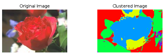
This section provides a simple example of performing classification using an autoencoder. An autoencoder is a type of neural network that specializes in learning a representation of the data, which can be used group or cluster a dataset into a small set of categories.
Use a small JPEG file for this example and cluster the image into five different categories based on the RGB pixel values. To read the image:
file = Filepath('rose.jpg', subdirectory=['examples', 'data'])
data = Read_Image(file)
IDL machine learning algorithms require the input data to be stored in a 2D array of size n x m, where n is the number of attributes and m is the number of examples. This example has three attributes (the red, green, and blue values per pixel), where the number of examples is the total number of pixels in the image. The data is a 3 x 227 x 149 array that you can reform to 3 attributes by 33823 examples by doing the following:
features = Reform(data, 3, (data.dim)[1]*(data.dim)[2])
As discussed in Prepare Data, define a normalizer that will transform the data. You can use any normalizer; this example uses IDLmlVarianceNormalizer:
Normalizer = IDLmlVarianceNormalizer(features)
Normalizer.Normalize, features
Now define the autoencoder, and determine how many layers to use. In this case, use two layers. Since there are three attributes, the sizes for the first and last layer must be 3. To cluster into five categories, the size of the middle layer will be 5.
Classifier = IDLmlAutoEncoder([3, 5, 3])
Note: To fine-tune your autoencoder, you can define an Activation Function for each layer. See Defining Activation Functions for more information.
Now train the model. During training, an autoencoder will learn how to produce the input image based on features. These internal features effectively become the clustered image:
Optimizer = IDLmloptGradientDescent(0.01)
p = Plot(Fltarr(2), title='Loss')
Loss = List()
for i=1, 300 do begin
Loss.Add, Classifier.Train(features, OPTIMIZER=Optimizer)
p.SetData, Loss.ToArray()
endfor
Note: Training a neural network requires the use of an optimizer. An optimizer helps the neural network adjust the learning rate during training based on how quickly the model converges to a solution. The optimizers are: IDLmloptAdam, IDLmloptGradientDescent, IDLmloptMomentum, IDLmloptQuickProp, and IDLmloptRMSProp.
Tip: An instance of an optimizer should not be reused to train a different model.
To obtain the clustered image, classify the input data:
result = Classifier.Classify(features)
Display the original image next to the cluster result:
!null = Image(data, title='Original Image', layout=[2,1,1])
!null = Image(Reform(result, (data.dim)[1], (data.dim)[2]), $
rgb_table=25, title='Clustered Image', layout=[2,1,2], /current)
Which results in an image that looks like this:
Regression
IDL provides three classes you can use for regression purposes:
This section provides a simple example of performing regression using a Feed Forward Neural Network model.
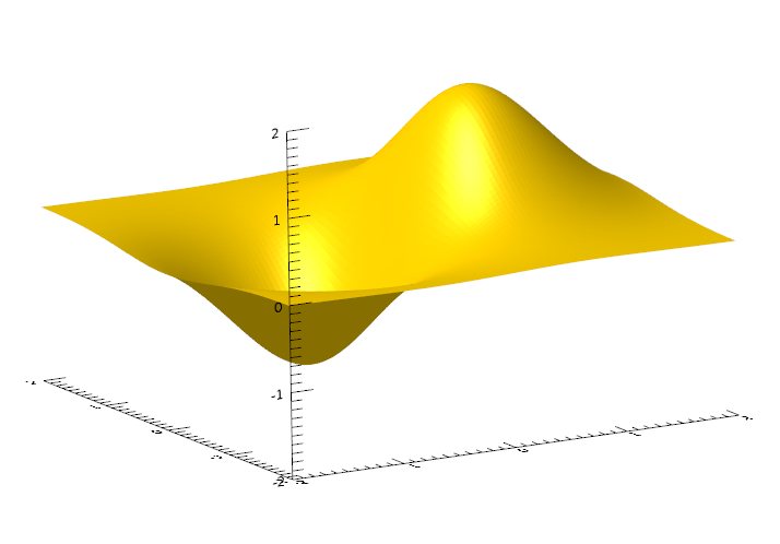
First, define an array with two attributes (x and y), and a particular shape for the model to learn:
size = 100
x = Findgen(size) / (size-1) * 4 - 2
y = Fltarr(size) + 1.0
xx = x # y
yy = Transpose(xx)
zz = 2.0/(exp((xx-0.5)^2+yy^2))-2.0/(exp((xx+0.5)^2+yy^2))
s = Surface(zz)
IDL machine learning algorithms require storing the input data in a 2D array of size n x m, where n is the number of attributes and m is the number of examples. In the example below, the number of attributes is 2 (the x and y components), where the number of examples is the total number of values in the array. Combine the xx and yy arrays into a 2D array with the following:
features = Transpose([[Reform(xx, size^2)], [Reform(yy, size^2)]])
scores = Reform(zz, size^2)
Now shuffle and partition the data into two groups: one group will be used for training, the other for testing. Make the groups the same size:
IDLmlShuffle, features, scores
part = IDLmlPartition({train:50, test:50}, features, scores)
As discussed in Prepare Data, define a normalizer that will transform the data. You can use any normalizer; this example uses IDLmlVarianceNormalizer:
Normalizer1 = IDLmlVarianceNormalizer(features)
Normalizer1.Normalize, features
The same applies to the model outputs. Unlike classification, where there are a finite and fixed set of outputs, the output of a regression is continuous, and it is important to keep it normalized.
Normalizer2 = IDLmlVarianceNormalizer(scores)
Normalizer2.Normalize, scores
Now define the neural network, and determine how many layers to use. In this case, use three layers. Since there are three attributes, the size for the first layer must be 3. For a regression problem, the size of the last layer will be 1, since you will not be classifying into different classes.
Model = IDLmlFeedForwardNeuralNetwork([2, 7, 7, 1], $
ACTIVATION_FUNCTIONS=[IDLmlafArcTan(), IDLmlafArcTan(), $
IDLmlafArcTan()])
Defining Activation Functions
Activation functions are important in machine learning. They allow neural networks (which by themselves are only linear systems) to introduce non-linearities, thus making them able to model more complex functions. IDL includes the following activation functions:
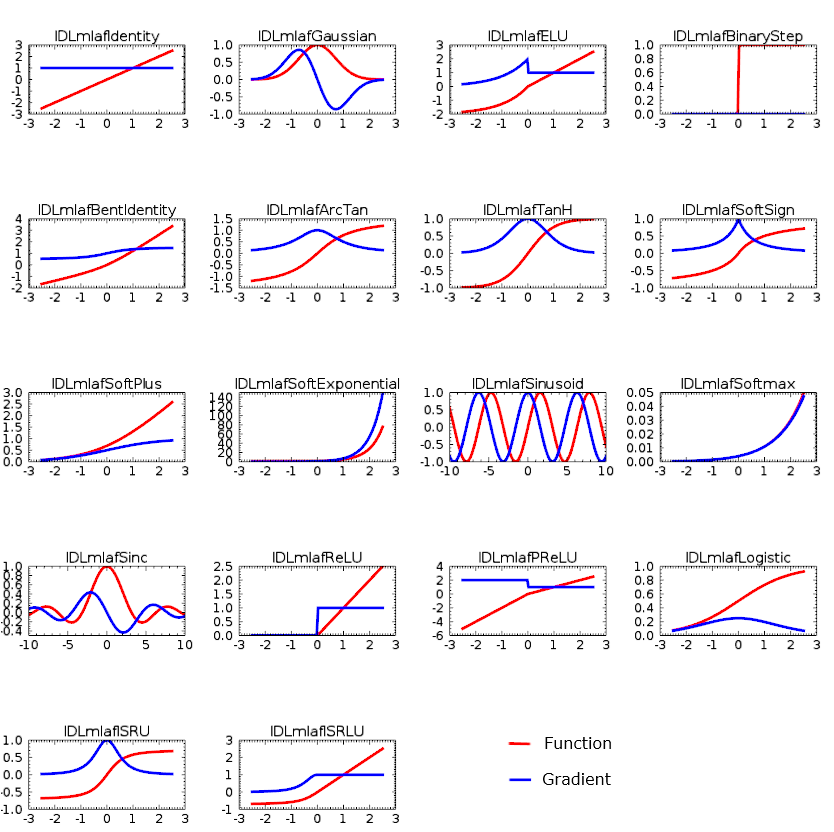
Choosing the right activation function for each layer is crucial to the accuracy of the neural network. There are very few guidelines; therefore, in most cases it is a trial and error method:
Optimizer = IDLmloptAdam(0.1)
Loss = List()
p = Plot(Fltarr(10), title='Loss')
for i=1, 300 do begin
Loss.Add, Model.Train(part.train.features, $
SCORES=part.train.scores, OPTIMIZER=Optimizer)
p.SetData, Loss.ToArray()
endfor
Note: Training a neural network requires the use of an optimizer. An optimizer helps the neural network adjust the learning rate during training based on how quickly the model converges to a solution. The following optimizers are available: IDLmloptAdam, IDLmloptGradientDescent, IDLmloptMomentum, IDLmloptQuickProp, and IDLmloptRMSProp.
Tip: An optimizer that is used to train one model should not be reused to train a different model.
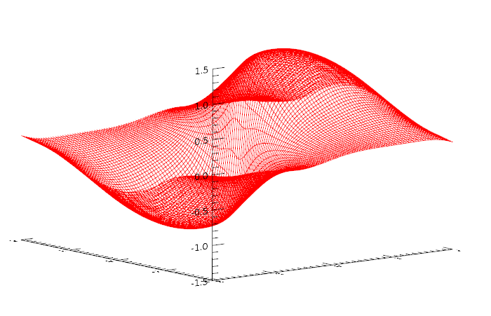
Now pass the entire x, y dataset through the model and see how well the output resembles the data it tried to learn:
data = Transpose([[Reform(xx, size^2)], [Reform(yy, size^2)]])
Normalizer1.Normalize, data
result = Model.Evaluate(data)
result2D = Reform(result, size, size)
!null = Surface(result2D, xx, yy, color=[255,0,0], style='mesh')
You can also use the Evaluate method to evaluate the accuracy of the model against the test data. This is returned by the LOSS keyword that will produce the RMSE (root mean square error) of the calculated results as compared to the actual scores:
!null = Model.Evaluate(part.test.features, SCORES=part.test.scores, $
LOSS=loss)
print, loss
The result is 0.0981930.
To use the model in a future IDL session without having to retrain it, you can save it to a file. Also save the normalizer, since you will have to renormalize your data too:
Model.Save, 'c:\tmp\model.sav'
Normalizer1.Save, 'c:\tmp\normalizer.sav'
To restore these in a future IDL session:
Model = IDLmlModel.Restore('c:\tmp\model.sav')
Normalizer = IDLmlNormalizer.Restore('c:\tmp\normalizer.sav')
See Also
IDL Machine Learning list of routines