Generate Point Clouds and DSM Tutorial
This tutorial shows how to generate point clouds and a digital surface model (DSM) from IKONOS satellite stereo imagery. You will view the resulting point clouds in the ENVI LiDAR Viewer and the resulting DSM in ENVI.
This tutorial requires a separate license for the ENVI Photogrammetry Module; contact your sales representative for more information.
The estimated time to complete this tutorial is one hour.
Generating point clouds uses a significant amount of memory. We recommend a minimum of 8 GB of RAM. Consider increasing the amount of RAM on your system if performance is an issue.
Files Used in this Tutorial
Tutorial files are available from our ENVI Tutorials web page. Click the IKONOS Stereo link to download the .zip file to your machine, then unzip the files. You will use the files listed below in the tutorial.
The files HobartIKONOS1.dat and HobartIKONOS2.dat are spatial subsets of IKONOS-2 stereo panchromatic images of Hobart, Tasmania, saved to ENVI raster format. For best results, you should process full scenes rather than spatial subsets. We created spatial subsets for this tutorial to save disk space and to shorten the processing time.
The scenes were acquired on 22 February 2003, 00:27:00 UTC. The pixel size is 1 meter with 11-bit radiometric resolution. They overlap in geographic coverage by at least 90 percent and contain rational polynomial coefficients (RPCs). Specific image characteristics are as follows:
|
File |
Description |
|
HobartIKONOS1.dat
|
A spatial subset of the GMTED2010 digital elevation model (DEM) at 7.5 arc-second resolution, covering the geographic area around Tasmania.
- Cross-scan acquired nominal ground sampling distance (GSD): 0.90 meters
- Along-scan acquired nominal GSD: 0.93 meters
- Scan azimuth: 180.05 degrees (reverse scan)
- Nominal collection azimuth: 329.4211 degrees
- Nominal collection elevation: 69.13697 degrees
|
|
HobartIKONOS2.dat
|
- Cross-scan acquired nominal GSD: 0.93 meters
- Along-scan acquired nominal GSD: 0.91 meters
- Scan azimuth: 180.05 degrees (reverse scan)
- Nominal collection azimuth: 235.7357 degrees
- Nominal collection elevation: 48.88442 degrees
|
IKONOS images are courtesy of DigitalGlobe.
Background
ENVI uses a dense image-matching algorithm that identifies corresponding points in two or more images of the same geographic area. For a given point in one image, it searches a two-dimensional grid of points in the second image. By having orientation data, the search is reduced to one dimension: along an epipolar line in the second image. A DEM imposes a constraint on the range of heights in the matching area, which constrains the length of the epipolar line. This reduces both the risk of false matches and the time in matching by reducing the search space. The success of the algorithm depends on the intersection angle and similarity between the images.
Point clouds generated from satellite stereo imagery are useful for DEM extraction over large geographic areas. While you can extract features such as buildings and trees to some extent, synthetic point clouds from satellite images are not meant for that purpose. Point clouds generated from aerial scanners are better suited for detailed terrain analysis and feature extraction, but their file sizes and cost are often prohibitive. ENVI generates synthetic point clouds from two or more images from different view points for 3D visualization, DEM extraction, and viewshed analysis over large areas.
Open and Display Images
- Start ENVI.
- Click the Open button
 in the ENVI menu bar. The Open dialog displays.
- Navigate to the folder where you downloaded the tutorial data. Use Ctrl-click to select the files HobartIKONOS1.dat and HobartIKONOS2.dat.
- Click Open. Both images are added to the view and the Layer Manager.
-
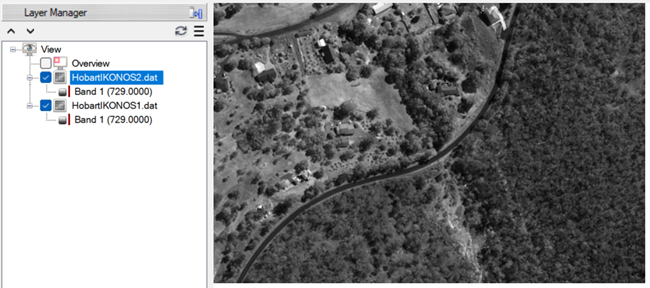
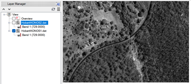
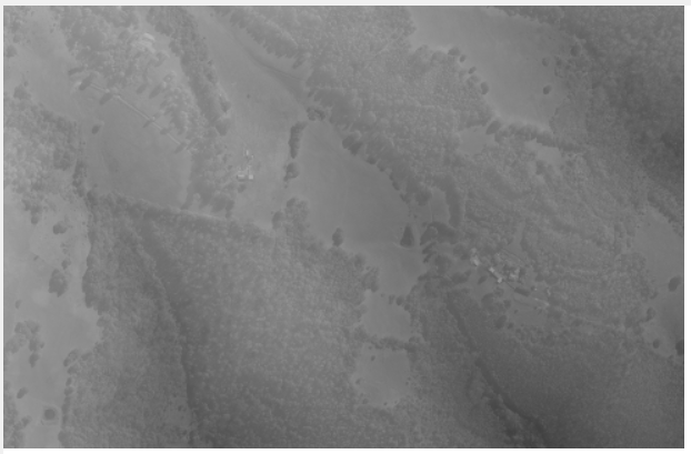
Uncheck the HobartIKONOS2.dat layer in the Layer Manager to view the underlying HobartIKONOS1.dat layer. By toggling between the two layers, you can see the differences in their view geometry. The following screen captures show an example:
Generate Point Clouds and DSM
- In the Toolbox, expand the Terrain category.
- Double-click Generate Point Clouds and DSM by Dense Image Matching.
- Click the Browse button
 next to the Input Rasters field.
- Click the Select All button, then click OK.
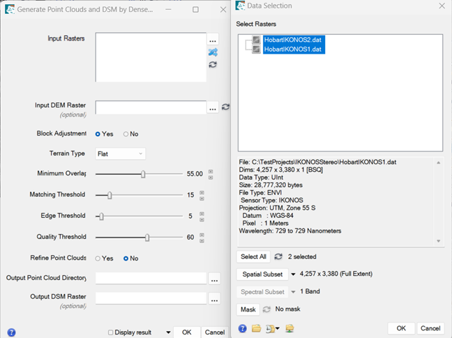
- In the Generate Point Clouds and DSM by Dense Image matching dialog, click the Browse button next to the Input DEM Raster field.
- Click the Open File button in the File Selection dialog.
- Navigate to the directory where you saved the tutorial data, and select the file HobartDEM.tif. Click Open.
- Click OK in the Data Selection dialog.
- Keep the default selection of Yes for Block Adjustment. Applying a block, or bundle, adjustment to satellite images refines the image geometry and improves the quality of the generated point clouds.
- From the Terrain Type drop-down list, select Mountainous. The input image contains mostly mountainous terrain.
- Leave the remaining parameters at their default values.
Tip: You do not have to perform this step in the tutorial, but you have the option to create a DEM with the ENVI LiDAR application after generating point clouds. If you were to create a DEM, you can select the Yes option for Refine Point Clouds option in the Generate Point Clouds dialog. This will smooth the point clouds, which will produce a smoother DEM.
- Choose an Output Point Cloud Directory to save the LAS point cloud files. Since this process will create several LAS files, consider creating a separate PointClouds directory to save them in.
- Enter a filename for the Output DSM Raster. The output will be in TIFF format.
- Enable the Display result check box.
- Click OK. A progress dialog appears.
Note: If you receive a "Failed to generate point clouds" error message, look for and remove the _JAVA_OPTIONS environment variable from your Windows system. In the Windows Start menu, type environment in the search bar. Select edit the system environment variables. Under the Advanced tab in the System Properties dialog, click the Environment Variables button. Select _JAVA_OPTIONS in the System variables list, and click the Delete button.
View the Digital Surface Model
- When the DSM image displays, press the F12 key on your keyboard to view its full extent.
- Click the Cursor Value icon
 in the ENVI toolbar. The Cursor Value dialog displays the pixel values for the crosshair location for all of the current layers, including the DSM and two IKONOS images. Note the Data line under the DSM file name. This is the DSM pixel value at the crosshair location. In this example, the value is 172.498901 meters:
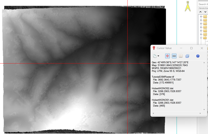
The DSM image has some artifacts along the edges where no data exists or where point clouds could not be generated.
- Close the Cursor Value dialog.
- Pan and zoom into the DSM image to explore it further. Use the Transparency slider in the ENVI toolbar to compare the DSM with the underlying IKONOS image (HobartIKONOS2.dat). You can see where the bright values in the DSM correspond to hills in the IKONOS image, and low DSM values correspond to valleys. The following figure shows an example with the DSM transparency set to 20% so that the DSM and IKONOS image are both visible:
View Point Clouds
- In the search window of the Toolbox, type lidar.
- Double-click the Launch ENVI LiDAR tool name that appears. The ENVI LiDAR application starts.
- From the ENVI LiDAR menu bar, select File > New Project. The Save As dialog appears.
- Navigate to the IKONOSStero folder you created and enter IKONOSProject as the filename. Click Save.
- A dialog appears that says, "Please select LAS or other data files to be imported into project." Click OK to close the dialog. The Open dialog appears.
- Navigate to your output directory from the previous section. Use Shift-click to select all of the .las files that were generated. Click Open.
- A dialog appears that says, "Do you want to import more raw material data files into the project?" Click No to close the dialog.
- A dialog appears with the current map projection details of the LAS files. Click Yes to use these values. ENVI LiDAR will now process the point clouds and generate its own digital surface model (DSM), which is different than the one you created in ENVI. This process can take several minutes.
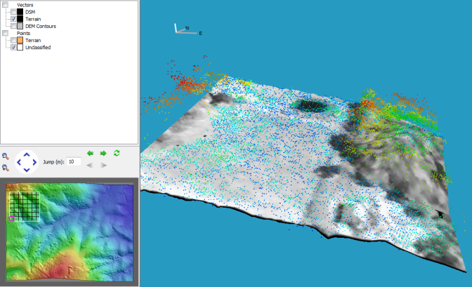
-
The rendered point clouds appear in the Main window (blue background). A thumbnail view of the DSM appears in the Navigate window (gray background).
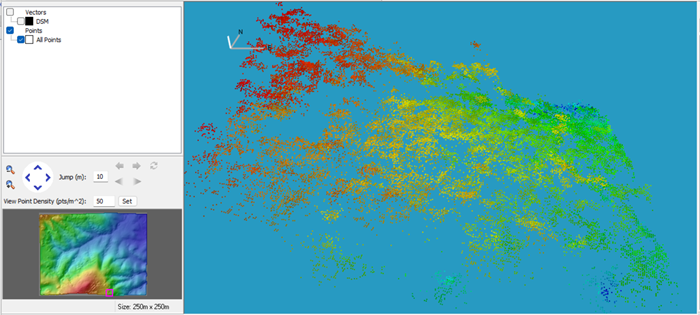
- In the Navigate window, click and drag to select an area to display in the Main window. A magenta box in the Navigate window indicates the selected area. Here is an example:
- Explore the point cloud image using these tips. Refer to the ENVI LiDAR Help for additional details.
- To zoom in and out, right-click and drag up or down across the view. Or use the mouse wheel.
- To pan, click both mouse buttons and drag in any direction across the image. Or use the arrow keys on your keyboard.
- To rotate the image along the x and z axes, click and drag across the view.
- To select the area to display in the Main window, click and drag on the DSM thumbnail in the Navigate window. The smallest selection size is 30x30 meters; if you select an area smaller than that range, the size automatically increases to 30x30 meters. The largest selection size is 2000x2000 meters.
- To save the current view so you can return to it later, select View > Save from the menu bar. Enter a Display Name in the Select Display Name dialog and click OK. To display a saved view, select View > Display from the menu bar and select the view from the Saved Views dialog.
- To create a screen capture of the current view that you can open later in graphics applications, press Ctrl+C on the keyboard. The Operations Log in the lower part of the application displays the location and name of the screen capture. Or select File > Screenshot to PowerPoint from the menu bar to capture the screen and launch PowerPoint presentation software (if it is installed on your machine).
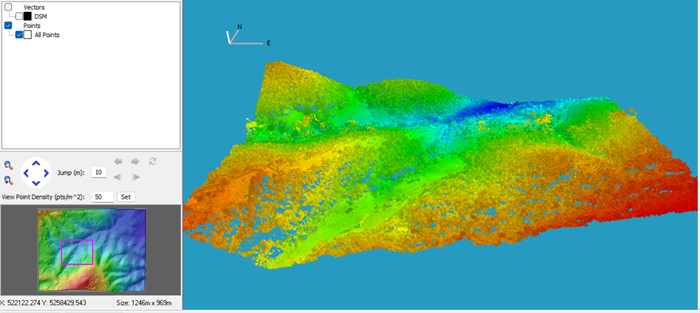
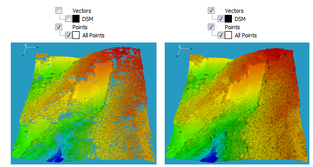
- Notice that some areas have patches of missing data; the blue background shows through these gaps. ENVI created a temporary DSM that can be used to interpolate the elevation data in these gaps. To view the DSM in the Main window, select the DSM option in the Layer Manager of ENVI LiDAR:
Generate a Density Map
You can generate a density map that shows the point density of the LiDAR raw data.
- Select Process > Generate Density Map from the menu bar. The Select Format dialog appears.
- From the Format drop-down list, select ENVI elevation format and click OK.
- The density map shows higher and lower density by variation in color. Move your cursor around the density map, and notice the Density value:
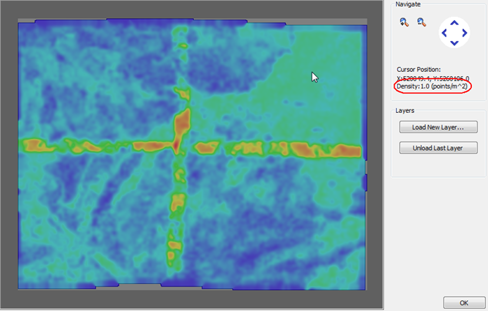
- The point density of this dataset ranges from approximately 0.1 to 4 points per square meter. In the urban area in the northeast corner of the density map, the average point density is 1 point per square meter. At this resolution, ENVI LiDAR can process buildings and trees; however, those results will likely contain many false readings. With more points per square meter and high-quality point clouds, ENVI LiDAR can more accurately identify features for extraction and avoid false readings.
- Click OK to close the density map.
Create Elevation Products
These steps show how to extract an orthophoto and DEM from the point cloud data.
- From the ENVI LiDAR menu bar, select Process > Process Data. The Project Properties dialog appears.
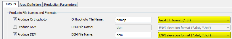
- Under the Outputs tab, select the options for Produce Orthophoto and Produce DEM. You will not create a DSM since you already created one in ENVI.
- Keep the default output formats for the orthophoto and DEM:
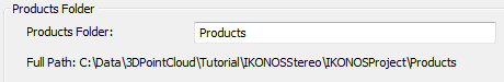
- Note the location of the Products folder. This is where the rasters will be created. The following figure shows an example:
- Select the Production Parameters tab.
- Click the DEM Advanced Parameters button:
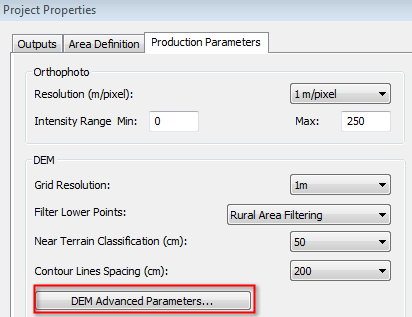
- In the DEM Advanced Production Parameters dialog:
- Enable the Variable Sensitivity Algorithm check box.
- From the DEM Sensitivity drop-down list, select 30 - Medium.
- Leave the default value of 2 for Constant Height Offset (cm).
- Click OK.
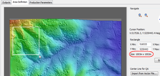
- Select the Area Definition tab.
- Click and drag the cursor to draw a box over some terrain that is approximately 1000x1000 meters, as shown by the Size field:
- Click the Start Processing button at the bottom of the Project Properties dialog. This process will take several minutes to complete. The Navigate window shows the progress by blocks; magenta-colored blocks indicate in progress, and white-colored blocks indicate completed. The Operations Log and the status bar of the Main window also show the progress.
- When processing is complete, a dialog appears that says, "Processing complete, entering QA Mode." Click OK to dismiss the dialog.
- By default, ENVI LiDAR automatically changes the display to QA Mode. This view shows an image display of the terrain. The image in the Navigate window is divided into grids.
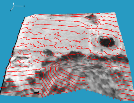
- Disable the Unclassified Points layer in the Layer Manager, and enable the DEM Contours layer to view contours over the terrain.
- From the ENVI LiDAR menu bar, select File > Preferences.
- In the Preferences dialog, change the DEM Contours Vector Color to a different color that is more visible (for example, red).
- Click OK in the Preferences dialog. The following figure shows an example of the DEM contours:
- From the ENVI LiDAR menu bar, select File > Launch Products in ENVI.
- In the Launch Generated Products in ENVI dialog, keep the default selections and click Launch. A new instance of ENVI appears with the DEM (dem.dat) and orthophoto (bitmap.tif) selected in the Layer Manager.
- When you are finished exploring the elevation products, close ENVI.
- The ENVI LiDAR project automatically saves. You can close the application and restart it later, and the project will open in the state where you left it.
This concludes the tutorial. If you have further questions about point cloud generation or ENVI LiDAR, please refer to ENVI Help.