This tutorial demonstrates how to create an orthorectified mosaic from two QuickBird multispectral images and a DEM of Phoenix, Arizona, USA. You will learn how to properly open the images and DEM in ENVI Classic, restore a ground control point (GCP) file, add new GCPs, add tie points, and define the parameters of the orthorectified product.
This tutorial requires the ENVI Photogrammetry Module; contact your sales representative for more information.
The ENVI Photogrammetry Module is a joint collaboration between NV5 Geospatial Solutions, Inc. and Spacemetric AB of Stockholm, Sweden. Spacemetric designed the underlying block-adjustment model, which provides a precision orthorectification solution for various sensors. For more technical information on Spacemetric’s orthorectification models, see their website at https://www.spacemetric.com/.
Files Used in This Tutorial
The files used in this example are available from our ENVI Tutorials web page. Click the Rigorous Ortho link to download the .zip file to your machine, then unzip the files to a directory named rigorous_ortho.
|
File |
Description |
|
005606990010_01_P008_MUL\05JUL*.TIF
|
QuickBird Level-1 multispectral imagery for Phoenix, AZ from 11 July 2005
|
|
005606990010_01_P011_MUL\05OCT*.TIF
|
QuickBird Level-1 multispectral imagery for Phoenix, AZ from 09 October 2005
|
|
phoenix_DEM_subset.tif
|
DEM subset of Phoenix, AZ, in GeoTIFF format
|
|
phoenixGCPs.pts
|
Ground control points (GCPs) for the 05JUL* QuickBird image (in the 005606990010_01_P008_MUL directory)
|
QuickBird files are courtesy of Maxar/DigitalGlobe.
Background
An orthorectified image (or orthophoto) is one where each pixel represents a true ground location and all geometric, terrain, and sensor distortions have been removed to within a specified accuracy. Scale is constant throughout the orthophoto, regardless of elevation, thus providing accurate measurements of distance and direction. Geospatial professionals can easily combine orthophotos with other spatial data in a geographic information system (GIS) for city planning, resource management, and other related fields.
RPC Orthorectification allows you to orthorectify images using rational polynomial coefficients (RPCs), elevation and geoid information, and optional ground control points (GCPs). However, RPCs and elevation information do not provide enough details to build a rigorous model representing the path of light rays from a ground object to the sensor.
The Rigorous Orthorectification tool allows you to build highly accurate orthorectified images by rigorously modeling the object-to-image transformation. The details of this transformation are mostly transparent to the user, which means you can quickly create orthorectified images without defining detailed model parameters.
The tool includes the ENVI Orthorectification Layout Manager, which helps you see the spatial coverage of images, DEMs, GCPs, and tie points, along with residual error vectors for each GCP. You can adjust your GCPs and tie points to improve the overall residual error for the orthorectified output. Automatic color balancing is available during the final output step.
Workflow
The figure below shows a typical orthorectification workflow. The required steps are:
-
Select input images and DEMs.
-
Build an adjustment model.
-
Select output parameters.
-
Rectify the input image(s) to produce the output image.
However, you will achieve the most accurate results by incorporating optional ground control points (GCPs) and tie points into the model, while iteratively reviewing the overall model error and editing points as needed to reduce the error. You can also optionally create and edit cutlines and set some basic parameters for the final output.
The shaded boxes represent workflow steps that have an associated wizard dialog to guide you through the process.
Select Input Images and DEM
Input images must be in their native format and directory structure, exactly as they are delivered by the data provider. The imagery must include all associated metadata and ephemeris data.
Open the image files before loading the images into the Orthorectification Wizard. Use the following steps:
- Start ENVI.
- From the menu bar, select File > Open. The Open dialog appears.
- Navigate to rigorous_ortho/005606990010_01_P008_MUL, and open 05JUL11182931-M1BS-005606990010_01_P008.TIF. The file appears in the Available Bands List. This is a multispectral image of Phoenix, Arizona, captured on 11 July 2005. This file will be referred to as the 05JUL* image throughout the rest of the tutorial.
- Select File > Open, navigate to rigorous_ortho/005606990010_01_P011_MUL, and open 05OCT09183407-M1BS-005606990010_01_P011.TIF. The file appears in the Available Bands List. It is a multispectral image of Phoenix, Arizona, captured on 09 October 2005. This file will be referred to as the 05OCT* image throughout the rest of the tutorial.
- Last, open the DEM subset file that was included in the tutorial data. Select File > Open, navigate to rigorous_ortho, and select the file phoenix_DEM_subset.tif. Click Open. This is a subset of a U.S. Geological Survey DEM from the Phoenix area. It is in a Geographic Lat/Lon projection with a WGS-84 datum.
Load Images and DEM into the ENVI Orthorectification Wizard
- In the ENVI Toolbox, select Geometric Correction > Orthorectification > Rigorous Orthorectification. The ENVI Classic display group opens with the images loaded, and the ENVI Orthorectification Layout Manager and the ENVI Orthorectification Wizard appear.
- In the Wizard (Step 1 of 5), click the
 button next to the Input Images field. The Select Input Files dialog appears.
- Use the Ctrl key to select both GeoTIFF images (05OCT* and 05JUL*). Click OK. The Select Sensor Type dialog appears.
- Select QuickBird, then click OK. The image filenames are listed in the Input Images field of the Wizard.
- Click the button next to the Input DEMs field. The Select Input Files dialog appears.
- Select Band 1 under phoenix_DEM_subset.tif, and click OK. The DEM filename is listed in the Input DEMs field of the Wizard.
- Click Next in the Wizard. After the images and DEMs load, their boundaries are shown in the Layout Manager.
The top of the Layout Manager shows the projection of the input images. The Map X/Y coordinates update as you move the cursor around the draw area (the black area that shows the different layers of data):
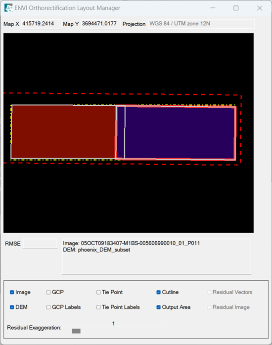
The DEM (shown with a red dashed box) surrounds the two QuickBird images. Use the DEM checkbox in the Layout Manager to turn on/off the DEM boundary.
The two QuickBird images overlap. The image boundaries are shown with solid grey boxes, and their interiors are filled with different colors. Use the Image checkbox in the Layout Manager to turn on/off the gray image boundaries in the Draw Area.
The yellow dashed box represents the default output area for the orthorectified product, which is currently selected to be the image boundaries. Use the Output Area check box in the Layout Manager to turn on/off the yellow boundary in the Draw Area.
As you move the cursor over an image boundary, the underlying image and DEM filename appear. In the area where both images overlap, both image filenames appear.
Use the scroll wheel on your mouse to zoom in or out. Or, right-click inside the draw area to select different zoom options. Click and drag the mouse to pan around.
Working with Ground Control Points
After you load the QuickBird images and DEM into the Wizard and click Next, the Wizard proceeds to the GCP Selection panel (Step 2 of 5), and a display group opens for the 05OCT* image. In the GCP Selection step, you will associate image pixels to points on the ground whose locations are known through a horizontal coordinate system and vertical datum. These points are called ground control points (GCPs).
The controls in this step of the wizard allow you to optionally restore GCP files, add new GCPs, and edit existing GCPs. Although selecting GCPs is an optional step in the overall workflow, you will achieve the most accurate orthorectified results by using GCPs and iteratively reviewing the overall RMS error.
Restore GCPs
For this tutorial, you will restore a set of GCPs that lie within the 05JUL* QuickBird image boundary (the left image as shown in the Layout Manager). DigitalGlobe, who provided the QuickBird images, also produced a set of GCPs for the entire Phoenix area, in Microsoft Excel format. However, Rigorous Orthorectification requires GCPs to be in a “Rigorous Orthorectification GCP” format. For more information, see the ENVI Classic Help.
The GCP file you are about to restore (phoenixGCPs.pts) was created by identifying those GCPs that fell within the 05JUL* QuickBird image boundary, then entering them one-by-one into the ENVI Orthorectification Wizard using map coordinates provided by DigitalGlobe. The GCPs were already in a Geographic Lat/Lon projection with WGS-84 datum (the same projection as the QuickBird images and DEM). The GCP file was then saved to ENVI format, using the Save GCPs button in the Wizard.
The first few lines in the GCP file (phoenixGCPs.pts) are the header lines, and they are preceded by semicolons. They list the input images you selected earlier. They currently only list the filenames, but the Rigorous Orthorectification GCP file format requires a full path to the image filenames. You will need to edit phoenixGCPs.pts to include the full path to the 05JUL* QuickBird image filename on your computer. As mentioned in the introduction, you should save a copy of the entire rigorous_ortho directory to your local drive, so that you can save your changes to the GCP file.
- Navigate to rigorous_ortho and open the file phoenixGCPs.pts in a text editor.
- Edit the third line that begins with FileName1 to include the full path to the 05JUL* image; for example:
Note: You do not need to edit the FileName0 line, since the GCP locations in phoenixGCPs.pts only pertain to the 05JUL* image (FileName1).
- Save the file phoenixGCPs.pts.
- When working with multiple input images, you need to specify which image corresponds to the GCPs you are about to restore or add. In the Wizard, select the 05JUL* image filename from the Active Image list:
The display group updates to show the 05JUL* image.
- Click the Load a New GCP File button
 in the Wizard. The Select GCP File dialog appears.
- Select the file phoenixGCPs.pts that you just edited and saved, and click Open. The GCP Selection panel shows "Number of Active Points: 14." The GCPs also appear in the display group and the Layout Manager.
Add New GCPs
The GCPs you just restored are all within the 05JUL* image, so now you should add some GCPs to the 05OCT* image (the right-most image as shown in the Layout Manager). Unfortunately, there are only two available GCPs for this area. But this is a realistic scenario in orthorectification: you may not always have adequate GCP coverage throughout your area of interest, or the GCPs may be unevenly distributed.
- In the GCP Selection panel, click the 05OCT* image filename:
- Click the Projection toggle button
 .
.
- Click DDEG. The Lat and Lon fields change so that you can enter map coordinates in decimal degrees.
-
Enter the following values in their respective fields in the GCP Selection panel, then click the Add Point button:
Lat: 33.41914515
Lon: -111.90030564
Image X: 1058
Image Y: 385
Elev: 329.81
After a few seconds, the new GCP appears in the display group and Layout Manager.
-
Enter the following values, then click the Add Point button:
Lat: 33.39088287
Lon: -111.89436526
Image X: 1279
Image Y: 1631
Elev: 333.136
- Click the Show List button in the GCP Selection panel.
The table in the GCP Selection panel should look as follows. The new GCP locations that you added are shown in rows 15 and 16. The Geographic Lat/Lon coordinates are converted into eastings and northings for this table.
Evaluate Residual Errors
The controls in the Layout Manager to evaluate the overall model error are a powerful feature of Rigorous Orthorectification. As you interactively add, edit, or remove GCPs and tie points, the entire model is recomputed on-the-fly and your results are immediately visible in the Layout Manager. Note the RMSE (root mean square error) field that lists the overall model error. The current value should be 58.873389.
-
Enable the Residual Image option in the Layout Manager. A contour map is added to the Draw Area, showing the residual error throughout the area based on your GCP data. Purple-to-blue areas indicate the lowest residual errors, and red-to-white areas indicate the highest errors.
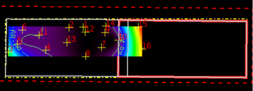
- Right-click inside the draw area, and select Zoom In until you can see the contour labels more closely. Click and drag the mouse to pan. From looking at this contour view, you can see that GCP #3 (in the far lower-left corner of the contour map) has a relatively high residual error.
- Scroll to the right of the GCP list until you see the Magnitude (m) field. The contour view of residual error is based on these relative magnitude values. There must be four or more GCPs in the list for this column to appear.
- Click on 3+ to select the row:
A diamond marker appears over the GCP. Its magnitude value is 200.33. This value is relatively high, compared to the magnitude values of other GCPs.
- Enable the Residual Vectors option in the Layout Manager.
- Increase the Residual Exaggeration value to 10.
- Disable the Residual Image option. Cyan-colored arrows originate from each GCP location, showing their error magnitudes and directions. The left side of the scene has the highest errors and, as expected, the GCP corresponding to ID #3 has the largest residual error vector.
.
In the next step, you will remove this GCP and see if the overall model improves.
- With Row 3+ still selected in the GCP list, click the Deletebutton. The entire model is recomputed, and the updated residual errors are shown in the Layout Manager. The row numbers are updated accordingly.
- What is the overall RMSE value now?
- Did the overall model improve after removing this GCP?
- Use the GCP list to look for other GCPs with relatively high magnitude values. In addition to removing GCPs, you can also interactively update their geographic location as follows:
- Select any GCP with a relatively high magnitude value.
- Open the Zoom window of the display group, which is centered over that GCP.
- Click the + button in the Zoom window to zoom in further.
- Click on a nearby pixel to move the crosshairs over that pixel.
- Click the Update button in the GCP list. This moves the GCP to the new pixel location and recalculates the overall model error.
- If the magnitude value for the GCP did not decrease, try a different pixel location and click Update.
- Repeat these steps with other GCPs as needed. The goal is to decrease individual GCP magnitude values and the overall RMSE value. This is an interactive process that involves much trial-and-error to produce the best results.
- Click Next in the Wizard to proceed to the Tie Point Selection panel.
Working with Tie Points
In this step, you can select pixels from both images that represent the same location on the ground. These pixels are called tie points. Although computing tie points is an optional step, tie points are an important component for computing the orthorectified model and account for most of the accuracy in the orthorectified product. In this exercise, you will add three tie points.
A display group appears with the 05OCT* image, while another display group contains the 05JUL* image. The Tie Point Selection panel shows the 05OCT* image as Image 1 and the the 05JUL* image as Image 2.
To save some time, the pixel coordinates for each tie point were already determined for you. This process involved identifying an object in the 05JUL* image (such as an intersection or building corner), zooming in, and using the Cursor Location/Value tool to record the image coordinates for that pixel. The same object was then identified in the 05OCT* image, and the fractional image coordinates for the corresponding pixel were recorded.
- Enter the following pixel coordinates that represent the first tie point, then click the Add Point button.
Image 1
Image X: 363, Image Y: 480
Image 2
Image X: 6736, Image Y: 512
- Enter the following pixel coordinates that represent the second tie point, then click the Add Point button.
Image 1
Image X: 490, Image Y: 1928
Image 2
Image X: 6860, Image Y: 1998
- Enter the following pixel coordinates that represent the third (and final) tie point, then click the Add Point button.
Image 1
Image X: 461, Image Y: 3086
Image 2
Image X: 6824, Image Y: 3186
The tie points are shown in the Layout Manager with magenta-colored “X” symbols:
- Click Show List in the Tie Point Selection panel to see the list of tie points.
- Before proceeding to the next step in the workflow, you should save your project. From the Wizard menu bar in the Tie Point Selection panel, select File > Save Project. The Select Project File dialog appears.
- Enter a filename and location for the project state, and click Save. The project state is saved in XML format. To restore your project later, select select File > Restore Project from the Wizard menu bar and select the XML file for your project. ENVI automatically opens all input files, DEMs, GCPs, and tie points, so you do not need to open them before restoring the project.
- Click Next in the Wizard to proceed to the Image Order and Cutline Selection panel.
Ordering Images and Defining Cutlines
In this optional step, you can define any areas between two or more overlapping images that you want to appear in the final output. With each input image, you perform two steps: (1) define the hierarchy of the image relative to the others, and (2) define an optional cutline for the image.
Use the Image Order list to define how multiple images are ordered in the final output. This list is populated with the image filenames you added to the workflow earlier. The image at the top of the list will be ordered first, followed by the second image, and so forth. Image ordering only pertains to areas of overlap between two or more images:
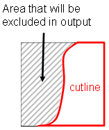
Cutlines are polygons that are used in combination with image ordering to define areas that you want to keep in the final output. A cutline is essentially an inclusion polygon, similar to a cookie cutter applied to one or more images. The following example shows a cutline for a single image:
Following is an example of applying a cutline to the first-order (top-most) image when you have multiple images.
For this tutorial, you will skip the process of ordering images and defining cutlines, by clicking Next. ENVI Classic will use the image frame as a cutline by default. The image frame is the area of usable image data, excluding any background pixels.
Define Output Parameters
Follow these steps:
- Enter an output filename and location for the orthorectified image. From the File Format drop-down list, select ENVI.
- Select the Auto Color Adjust option to perform automatic color balancing.
- Leave the default Pixel Size as 2.47400 m.
- In the Post Processing Reprojection section, leave the default projection of UTM Zone 12, WGS-84. ENVI Classic will use the pixel sizes of the input QuickBird images, to determine the X and Y pixel size of the orthorectified image.
- Click the Preview button to see a preview of the orthorectified image.
- Select the Display Result option to display the image after it has been created.
-
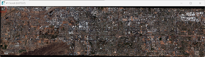
Click Finish to create the orthorectified image. This process will take a long time, as the two QuickBird images are very large. Following is a true-color version of the output mosaic as it appears in the Scroll window:
Optional Step
If you have some extra time, you may want to experiment with skipping the steps of adding GCPs and tie points altogether, then re-running the orthorectification process. Compare the RMSE value of the overall model with no GCPs or tie points.
GCPs and tie points should have a quality that is consistently better than the initial accuracy of the sensor model; this varies with data type and vendor. For example, mid-latitude QuickBird scenes of a relatively flat area may provide an accurate orthorectification without the use of GCPs or tie points.