SPHER_HARM

The SPHER_HARM function returns the value of the spherical harmonic Y_lm(θ,φ), which is a function of the longitude φ and the colatitude θ on a sphere (the colatitude is 90°–latitude). The degree l and order m have the following constraints: –l ≤ m ≤ l, l ≥ 0.

The spherical harmonics are related to the associated Legendre polynomial by:

For negative m the following relation is used:

where * represents the complex conjugate.

This routine is written in the IDL language. Its source code can be found in the file spher_harm.pro in the lib subdirectory of the IDL distribution.

Syntax

Result = SPHER_HARM( Theta, Phi, L, M, [, /DOUBLE] )

Return Value

SPHER_HARM returns a complex scalar or array containing the value of the spherical harmonic function. The return value has the same dimensions as the input arguments Theta and Phi. If one argument (Theta or Phi) is a scalar and the other argument is an array, the function uses the scalar value with each element of the array, and returns an array with the same dimensions as the input array.

If either Theta or Phi are double-precision or if the DOUBLE keyword is set, the result is double-precision complex, otherwise the result is single-precision complex.

Arguments

Theta

The value of the polar (colatitudinal) coordinate θ at which Y_lm(θ,φ) is evaluated. Theta can be either a scalar or an array.

Phi

The value of the azimuthal (longitudinal) coordinate φ at which Y_lm(θ,φ) is evaluated. Phi can be either a scalar or an array.

L

A scalar integer, L ≥ 0, specifying the order l of Y_lm(θ,φ). If L is of type float, it will be truncated.

M

A scalar integer, –L≤M≤L, specifying the azimuthal order m of Y_lm(θ,φ). If M is of type float, it will be truncated.

Keywords

DOUBLE

Set this keyword to force the computation to be done in double-precision arithmetic.

Example

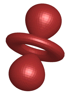
This example visualizes the electron probability density for the hydrogen atom in state 3d0. (Feynman, Leighton, and Sands, 1965: The Feynman Lectures on Physics, Calif. Inst. Tech, Ch. 19). The first part of this example defines the data and converts it from rectangular to spherical:

; Define a data cube (N x N x N)

n = 1511L

a = 60*FINDGEN(n)/(n-1) - 29.999  ; [-1,+1]

x = REBIN(a, n, n, n)              ; X-coordinates of cube

y = REBIN(REFORM(a,1,n), n, n, n)  ; Y-coordinates

z = REBIN(REFORM(a,1,1,n), n, n, n); Z-coordinates

; Convert from rectangular (x,y,z) to spherical (phi, theta, r)

spherCoord = CV_COORD(FROM_RECT= $

 TRANSPOSE([[x[*]],[y[*]],[z[*]]]), /TO_SPHERE)

phi = REFORM(spherCoord[0,*], n, n, n)

theta = REFORM(!PI/2 - spherCoord[1,*], n, n, n)

r = REFORM(spherCoord[2,*], n, n, n)

; Now compute the electron probability density and radial component.

; Find electron probability density for hydrogen atom in state 3d0

; Angular component

L = 2   ; state "d" is electron spin L=2

M = 0   ; Z-component of spin is zero

angularState = SPHER_HARM(theta, phi, L, M)

; Radial component for state n=3, L=2

radialFunction = EXP(-r/2)*(r^2)

waveFunction = angularState*radialFunction

probabilityDensity = ABS(waveFunction)^2

SHADE_VOLUME, probabilityDensity, $

 100*MEAN(probabilityDensity), vertex, poly

oPolygon = OBJ_NEW('IDLgrPolygon', vertex, $

 POLYGON=poly, COLOR=[180,50,50])

XOBJVIEW, oPolygon

The results are shown in the following figure (rotated in XOBJVIEW for clarity):

Version History

5.4	Introduced