ENVI Machine Learning offers three categories of machine learning. This section provides background on the categories, and the algorithms used in each.
See the following sections:
Supervised Classification
For Supervised Classification, you label data as ROIs regions of interest, and input the labeled data to one of six classification algorithms. Providing examples of known features of interest is why the algorithms described in this section are considered supervised.
Extra Trees Classification
The Extra Trees algorithm (also known as Extremely Randomized Trees) consists of multiple decision trees like Random Forest. It is similar to Random Forest, with a difference in time complexity and randomness. Extra Trees uses the entire original dataset, and constructs trees over every observation with different subsets of features. Extra Trees is faster because it does not look for the optimal split at each node; it instead does it randomly. The results are similar to Random Forest, but it takes less time to get the result.
Use Extra Trees to identify features that matter the most.
Advantages
-
Samples entire dataset
-
Nodes are split randomly reducing bias
-
Low variance, not heavily influenced by certain features
-
Faster since nodes are split randomly
-
Supports one or more features
Disadvantages:
-
Time complexity, slow when forest become large
-
Produces larger models compared to other algorithms
-
Not suitable for linear data with many sparse features
Random Forest Classification
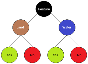
The Random Forest algorithm consists of multiple decision trees over the duration of training, using different subsets of the training data. It is similar to Extra Trees, with a difference in time complexity and randomness. Random Forest grows and combines multiple decision trees to create a forest. A decision tree can be viewed as a flow chart that branches out into different possible outcomes.
Advantages:
-
Low risk of overfitting to the dataset
-
Efficient with large datasets
-
Better accuracy than other algorithms
-
Robust to outliers
-
Implements optimal node splits improving the predictive capability of distinct trees in the forest
-
Supports binary and multiclass
Disadvantages:
-
Time complexity, slow when forest becomes large
-
Biased when dealing with categorical variables
-
Produces larger models compared to other algorithms
-
Not suitable for linear data with many sparse features
K-Neighbors Classification
K-Neighbors is a clustering algorithm that assigns a class label to a data point based on the label’s closest neighbors. KNN is a lazy learning algorithm because it does not perform training when you provide training data. Instead, it stores the data and builds the model once a query is performed on the dataset.
Advantages:
-
Simple and easy to understand
-
Sensitive to outliers and complex features
-
Does not make any assumptions, may reveal hidden data points
-
Sensitive to complex data
-
Non-linear performance
Disadvantages:
-
Time complexity, calculates the proximity between each neighboring values
-
Makes no assumptions treating all attributes as equally important
-
Consumes both the CPU and RAM storing all values in memory
-
Not ideal for large datasets with many classes
Linear SVM Classification
The Linear Support Vector Machine algorithm finds the minimum margin linear solution. Support vectors are data points closest to a hyperplane, and data points are used to determine the dividing line. The hyperplane is a decision space divided between a collection of features with various class assignments. Margin is the distance between two lines on the closest data points of various classes.
Use the linear kernel when the number of features is larger than the number of observations.
Advantages:
-
Performs well in high-dimensional space with good accuracy
-
Requires less memory only using a portion of the data
-
Performs decent with large gaps between classes
-
More useful when the number of dimensions exceeds the number of samples
-
Memory efficient
Disadvantages:
-
Takes a long time to train, not ideal for large datasets
-
Not able to distinguish overlapping classes
-
Performs poorly when the number of features of each data point exceeds the number of training samples
Naive Bayes Classification
The Naive Bayes algorithm uses the Bayes’ Theorem to naively calculate probabilities for each simplified hypothesis, making calculations easy to control or influence. Naive Bayes makes assumptions that all classes are independent, given the target values. This algorithm works well when assumptions made do not hold up.
Advantages:
-
Works well with minimal data
-
May converge faster than other discriminative models
-
Handles irrelevant features
-
Supports one or more features
-
Produces smaller models than other algorithms
Disadvantages:
-
Expects features to be independent to each other
-
Features in a large population may zero out when a sample does not represent the population well
-
Possible data loss when continuous variables are binned to extract discrete values from features
RBF SVM Classification
The Radial Basis Function Support Vector Machine algorithm tries to find the width of margin between classes using a nonlinear class boundary. It is considered a powerful kernel in the SVM family of classifiers. It determines the best hyperplane and maximizes the distance between points.
Use the Gaussian kernel when the number of observations is larger than the number of features.
Advantages:
Disadvantages:
• Training time is long; not ideal for large datasets
Anomaly Detection
For Anomaly Detection, you label non-anomalous data as ROIs regions of interest and provide the labeled data to one of two available classifiers. Anomaly Detection is a data pre-processing/processing technique used to locate outliers in a dataset. Outliers are features that are considered not normal compared to the known feature in a dataset. For example, if water is the known feature, anything that is not water would be considered an outlier/anomaly. Using minimal labeled pixels and ENVI tools such as Classification Aggregation, you can easily identify anomalies with minimal effort in labeling.
Isolation Forest Classification
The Isolation Forest algorithm uses binary trees to detect anomalies in data. Higher anomaly scores are given to data points that require fewer splits. Isolation Forest is a matching algorithm; anomalous data points that are few in number are considered rare. As a result, anomalous pixels are isolated from what is considered a normal pixel.
Advantages:
-
Smaller sample size works better, reduces the amount of labeling required
-
Less computation by avoiding distance and density calculations
-
Low memory requirement
-
Able to scale up and support large datasets and high-dimensional problems
Disadvantages:
Local Outlier Factor Classification
The Local Outlier Factor algorithm measures the local deviation of a given pixel with respect to its neighbors. A local outlier is determined by assessing differences of pixel values based on the neighborhood of pixels surrounding it.
Advantages:
Disadvantages:
-
Time complexity - longer training sessions, but faster than Isolation Forest
-
The local outlier factor scores for a given point being considered as an outlier may vary
-
Higher dimensions the detection accuracy is affected
Unsupervised Classification
Unsupervised Classification is helpful for data science teams who are unfamiliar with a particular scene and its features. This has the advantage of categorizing unknown similarities and differences in the data by grouping alike features. Having a good sense of what might be in the data can help fine-tune results. The number of classes requested before training determines the number of output classes/features.
BIRCH Classification
BIRCH (Balanced Iterative Reducing and Clustering using Hierarchies) is an unsupervised data mining algorithm used to achieve hierarchical clustering over datasets.
Advantages:
-
Saves time by not requiring labeled data
-
Dynamically clusters multi-dimensional data points to generate the best quality clusters
-
Efficient with large datasets
Disadvantages:
-
Time complexity, longer training sessions
-
High memory usage
-
Convergence is not guranteed
-
User must make sense of the identified features
-
User must tune the number of output classes to capture all features
Mini Batch K-Means Classification
Mini Batch KMeans is a variant of the KMeans algorithm, using mini batches to reduce the computation time while still attempting to optimize the same objective function. Mini batches are subsets of the input data, randomly sampled in each training iteration. These mini batches drastically reduce the amount of computation required to converge to a local solution.
Advantages:
-
Saves time by not requiring labeled data
-
Efficient with large datasets
-
Guarantees convergence
-
Generalizes to clusters with different shapes and sizes
-
Easily adapts to new examples
Disadvantages:
-
Time complexity, longer training sessions
-
Clustering of outliers where a single outlier may become its own cluster instead of being ignored
-
Has trouble clustering when density and size vary
-
Becomes less effective at distinguishing between examples as dimensions increase and the mean distance between examples decrease
-
User must make sense of the identified features
-
User must tune the number of output classes to capture all features