In this tutorial you will use ENVI Machine Learning to train an anomaly detection model to find anomalous features in an aerial image. You will learn how to set up an ENVI Machine Learning labeling project, train, classify, and post process your result to clearly identify anomalies. Time to complete 30 - 60 minutes.
See the following sections:
System Requirements
The steps for this tutorial were successfully tested with an Intel® Xeon® W-10855M CPU @ 2.80GHz 2.81GHz was used to run this tutorial (not required). Intel CPUs are recommended for performance gains due to the use of Intel libraries, but are not required.
Files Used in This Tutorial
Sample data files are available on our ENVI Tutorials web page. Click the "Machine Learning" link in the ENVI Tutorial Data section to download a .zip file containing the data. Extract the contents to a local directory.
The files for this tutorial are in the machine_learning\anomaly subdirectory.
The image used for this tutorial was provided by the National Agriculture Imagery Program (NAIP) (https://naip-usdaonline.hub.arcgis.com/). Images are in the public domain.
The image is a subset of the Los Angeles harbor containing multiple ships. This is a four band data (red/green/blue/NIR) with a spatial resolution of 1-meter ground sample distance (GSD).
|
File |
Description |
|
NAIP_LAHarbor_Subset.dat
|
NAIP image (6,519 x 4,568 pixels) used for training and classification
|
Background
Anomaly detection is a data pre-processing/processing technique used for locating outliers in a dataset. Outliers are features that are considered not normal compared to the known feature in a dataset. For example, if water is the known feature, anything that is not water would be considered an outlier/anomaly.
ENVI Machine Learning anomaly detection accepts a single background feature during training. This feature represents pixels that are considered normal for the entire dataset. Any pixel not considered normal during classification will be considered anomalous. A background feature for a given dataset is prepared during the labeling process prior to training.
Labeling data is critical in generating a good anomaly detector, this is true for most types of classifiers, especially for anomaly detection. For example, if labeled pixels that belong to an anomalous target are associated with the background feature, this will likely produce an inferior model.
Use Cases
- Identify anomalous features in imagery.
- Pre-processing step for generating training data in a different classification domain, such as deep learning.
Anomaly detection involves three, optionally four processes:
- Identify a background feature of common normality throughout the dataset, and draw ROIs around it. This is the labeling process.
- Perform training using labeled data to produce a model.
- Perform classification using the trained model, which generates a classification raster.
- Optionally, clean up false positives.
ENVI Machine Learning offers two types of anomaly detectors, Isolation Forest, and Local Outlier Factor.
- Isolation Forest is a matching algorithm, anomalous data points are few and considered rare. As a result, anomalous pixels are isolated from what is considered a normal pixel.
- Local Outlier Factor is an algorithm that measures the local deviation of a given pixel with respect to its neighbors. A local outlier is determined by assessing differences of pixel values based on the neighborhood of pixels surrounding it.
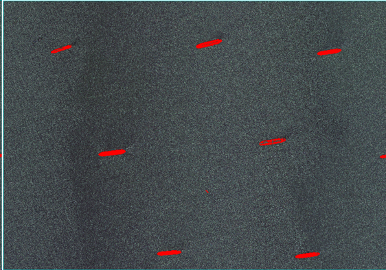
In this tutorial, you will train a model to detect all nine ships in a harbor as anomalous objects; for example:
Label Raster with ROIs
To begin the labeling process, you need at least one input image from which to collect samples of the image's dominant feature. Unlike traditional labeling, where you select objects or pixels of interest, anomaly detection requires the opposite approach. For this tutorial, water is the dominant feature and is what will be labeled as background. The image(s) you choose will be the training rasters. The images can be different sizes, but they must have consistent spectral and spatial properties. You will label the training rasters using ENVI ROIs, and the easiest way to do this is to use the Machine Learning Labeling Tool. Follow these steps:
Set Up a Labeling Project
- Go to the directory where you saved the tutorial files, and create a subfolder called Project Files.
- Start ENVI.
- In the ENVI Toolbox, expand the Machine Learning folder, and double-click Machine Learning Labeling Tool.
- Creating a project with the labeling tool will help organize all of the files associated with the labeling process. This includes the training rasters and associated ROIs.
-
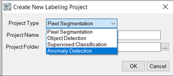
Select File > New Project from the Machine Learning Labeling Tool menu bar. Click the Project Type drop list and select Anomaly Detection.
- In the Project Name field enter Water.
- Click the Browse button
 next to Project Folder and select the Project Files directory you created earlier, click Select Folder.
- Click OK.
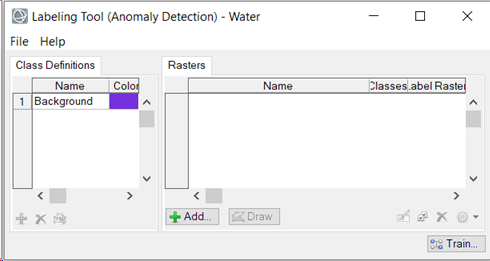
When you create a new Anomaly Detection project, the class definition Background is automatically created. You will not be able to add additional labels, and the label Background will be used to identify water. ENVI will create subfolders for each training raster you select as input. Each subfolder will contain the ROIs and training rasters created during the labeling process.
Add Training Rasters
- Click the Add
 button below the Rasters section of the Labeling Tool. The Data Selection dialog appears.
- Click the Open File button at the bottom of the Data Selection dialog.
- Go to the directory where you saved the tutorial data. In the machine_learning\anomaly folder select NAIP_LAHarbor_Subset.dat, then click Open.
- Select the image, if not already selected, in the Data Selection dialog, then click OK.
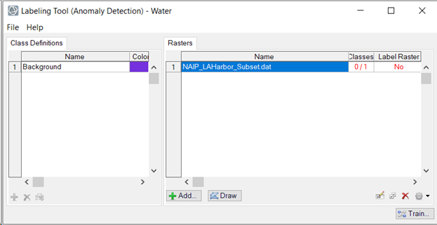
The training raster is added to the Rasters section of the Labeling Tool. The table in this section has two additional columns: "Classes" and "Label Raster." Each "Classes" table cell shows a red-colored fraction: 0/1. The "0" means that none of the class labels have been drawn yet. The "1" represents the total number of classes defined. The "Label Raster" column shows a red-colored "No" indicating that no label rasters have been created yet.
Label Water Pixels
It is important to be specific when labeling data for anomaly detectors (quality over quantity). Labeling too few pixels might not provide enough information to find all anomalous targets, while labeling too many pixels can result in longer classification run times. And if pixels that belong to an anomalous target are labeled, it will result in confusion and information loss.
- In the Labeling Tool select NAIP_LAHarbor_Subset.dat, if not already highlighted.
- Click the Draw button. The image is displayed. The Region of Interest (ROI) Tool opens. The ROI Name should be Background and its color should be purple. Move the Machine Learning Labeling Tool out of the way of the view, but do not close it.
- In the Layer Manager, select NAIP_LAHarbor_Subset.dat to make it the active layer.
-
Click the Stretch Type drop-down list in the ENVI toolbar and select Equalization. This stretch will allow colorized pixels to stand out for easier selection while labeling.
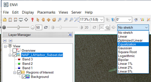
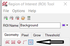
-
In the Region of Interest (ROI) Tool, select the Geometry tab and click the Point icon (highlighted in blue in the following image).
-
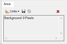
Click the Report Area of ROIs icon  . The Area section expands at the bottom of the Region of Interest (ROI) Tool dialog. This will show a count of how many pixels have been accepted for the Background class. The count populates when you accept the labeled pixels.
- In the Go To field in the ENVI toolbar , enter these pixel coordinates: 5480p,9276p. Be sure to include the “p” after each value. Then press the Enter key on your keyboard. The display centers over an area where the water has a darker greenish color.
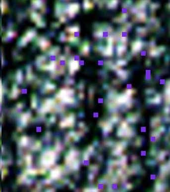
- In the ENVI toolbar, click in the Zoom drop-down list, enter 1200 in the field, then press Enter. The display zooms in 1200% (12:1) This zoom level is very pixelated, but this is needed to select specific colors of pixels.
-
Click on 25 pixels of different colors to label them. Try to get as many different color pixels as possible. A purple + icon will appear where you clicked.
Note: Do not label green and white pixels; these colors also represent pixel color values on some of the ships in the image.
To accept the selected ROI points, press the Enter key.
The purple + icons will become purple boxes after being accepted.
.
-
Use the three pixel coordinates below to label a total of 75 more pixels in the image (25 per coordinate set). Verify the NAIP_LAHarbor_Subset.dat layer is selected in the Layer Manager before you enter the coordinates in the Go To field.
For each coordinate set below, label 25 pixels, then press Enter to accept the ROIs.
7334p,10161p
9934p,9389p
7920p,11849p
-
When you have finished labeling, the Region of Interest (ROI) Tool Area should now show Background: 100 Pixels.
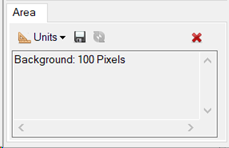
Leave the Region of Interest (ROI) Tool open. Labeling is now complete, and you can begin the training process.
Train an Anomaly Detection Model
For this tutorial you will use the Local Outlier Factor algorithm, which measures the local deviation of a given pixel with respect to its neighbors. A local outlier is determined by assessing differences of pixel values based on the neighborhood of pixels surrounding it.
- Click the Train button at the bottom of the Labeling Tool. The Train Machine Learning Model dialog appears. You can click the Help button
 at the bottom of the Train Machine Learning Model dialog. This provides a descriptions of the available parameters. When you are finished, click Close to close the Help dialog.
- Optionally provide a Description for the model.
- Leave the default Leaf Size at 30.
- Click the Browse button next to Output Model. The Select Output Model dialog appears.
- Choose an output folder and name the model file Ships.json, then click Save.
-
Click OK in the Train Machine Learning Model dialog.
In the Machine Learning Labeling Tool, the "Label Raster" column updates with "OK" for all training rasters, indicating that ENVI has automatically created labeled rasters for training. The generated training rasters contain a single row of spectra collected from all ROI labeled points with as many bands as the input raster in addition to a label band.
- Training will take a few seconds to complete, and a progress dialog displays.
-

The training step is complete. Now you can begin the classification process.
Perform Classification
Now that you have a model that was trained to differentiate against water pixels, you will use the model on the same raster to identify pixels that are not water. For this tutorial, the model generated is not generalized, and likely would not produce good results with other unseen imagery. You can train with multiple labeled rasters with ENVI Machine Learning, using the same labeling and training process provided in this tutorial.
- Close the ROI Tool and the Labeling Tool as they are no longer needed. The image will no longer be displayed after closing the Labeling Tool.
- Go to the ENVI Toolbox, expand the Machine Learning folder and double-click Machine Learning Classification. The Machine Learning Classification dialog appears.
- Click the Browse button next to Input Raster field. The Data Selection dialog appears.
- Click the Open File button
 and select NAIP_LAHarbor_Subset.dat, then click OK.
- Click the Browse button next to Input Model field. The Please Select a File dialog appears.
- Go to the location where you saved Ships.json, and click Open. The model file is opened and additional information displays below the Input Model field.
- Click Full Info to display model metadata. The Ships.json dialog opens, displaying information about the model. Once finished, click the X in the top right of the window to dismiss the Metadata dialog.
- Leave the Normalize Min and Max options blank; this information will be provided by the models scale factor values. Normalization reflectance values may differ from image to image. Min and Max are optionally available for cases where a generalized model is capable of classifying new imagery and the scale factors differ.
- Click the Browse button next to Output Raster. The Select Output Raster dialog appears.
- Go to the location where you created your workspace. Enter file name classification.dat, then click Save.
- Leave the Display result check box enabled.C
- Click OK. The Machine Learning Classification progress dialog displays. Classification should take from 30 – 60 seconds, depending on the system. Times may vary. When classification completes, the classification raster is displayed.
-
In the Layer Manager, right-click on Classification.dat and select Zoom to Layer Extent.
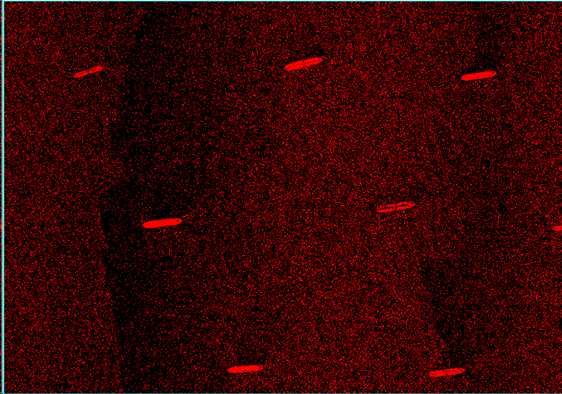
- At first glance you will notice the image is very noisy; this is a result of using minimal data (100 pixels). Using more labeled pixels as input to training can produce cleaner results, but at the cost of significantly longer classification times. Even with more trained pixels the result will still contain noise and likely require post processing to clean it up.
Classification is now complete, and you can begin post processing the classification result.
Post Processing
Now that you have performed classification, the next step is to clean up the result. For this tutorial, we know the ships are the anomalies in the scene. The goal of post processing will be to remove all water pixels, leaving only the ships. You can accomplish this using ENVI’s Classification Aggregation Tool.
- In the ENVI Toolbox Search field, type Aggregation, then double-click to select Classification Aggregation. The Classification Aggregation dialog appears.
- Click the Browse button next to Input Raster. The Data Selection dialog appears.
- Select the classification.dat raster produced during the classification process, and click OK.
- In the Minimum Size field, change the value to 500.
- Leave the default at Yes forAggregate Unclassified Pixels.
- Optionally, click the Browse button next to Output Raster. The Select Output Raster dialog appears. Enter the path and name of the output raster. If you leave this field blank, a temporary filename will be used instead.
- Leave the Display result check box enabled.
- Click OK. The Classification Aggregation Task progress dialog appears. This task will take 20 – 30 seconds to complete, depending on your system.
-
When Classification Aggregation completes, the result will be displayed. You will notice some pixels are missing from the ship interiors, this is a result of similar pixels being labeled.
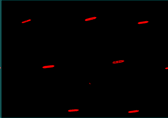
A Closer Look
The classification scene shows eight large ships and one tiny smudge toward the bottom center. Upon closer evaluation you will notice the small anomalous detection is indeed another ship.
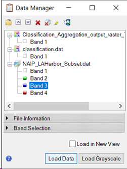
- Click the Data Manager button
 in the top left of the ENVI toolbar. The Data Manager dialog appears.
-
On raster NAIP_LAHarbor_Subset.dat, select bands in the order 4, 2, 3, then click Load Data. This will load the original raster as the first image in the Layer Manager. Selecting the order of bands as NIR=4 for red, 2 for blue, and 3 for green will display with the water appearing more natural than the default of 3, 2, 1 band order.
- In the Layer Manager, select and drag the Classification_Aggregation_output_raster*.dat above raster NAIP_LAHarbor_Subset.dat.
-
The Layer Manager should display the following order:
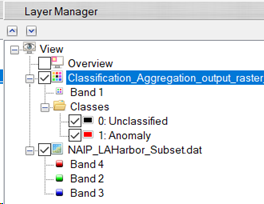
- In the Layer Manager under Classification_Aggregation* Classes, deselect class 0: Unclassified.
-
Zoom in on the smallest anomaly toward the bottom center of the display. If your mouse has a middle scroll wheel, this is the easiest way to zoom in. Or, you can use ENVI controls to zoom in by doing the following:
-
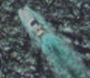
Select the Zoom drop-list and select 400% (4:1). The display zooms into the smallest anomaly at 400%. You should see something similar to image below, results may vary.
-
In the Go To field, enter coordinates 7389p,10988p and press Enter. The display centers over the smallest anomaly detected.

-
Using the Transparency tool in the ENVI toolbar, move the slider to the right. On close inspection, you can see this anomaly is also a ship. Water trails from the boat’s propellers are also classified as anomalous. Including labeled pixels of the water trails could help fine tune or worsen the results. Note, if you want to try this, you may need to reduce the Minimum Size when post processing with Classification Aggregation. This would be required if the small detection drops below the initial 500 pixels you used in the post processing step.
- When you are finished, exit ENVI.
Final Comments
In this tutorial you learned how to extract features at the pixel level using ENVI’s Machine Learning Labeling Tool. You learned that minimal Labeling was required to produce timely results with anomaly detection. You learned that ENVI tasks can be leveraged for Machine Learning processing. Using the same approach described in this tutorial, using multiple rasters, it is possible to produce a reusable generalized model for similar imagery.
In conclusion, machine learning technology provides a robust solution for learning complex spectral patterns in data, meaning that it can extract features from a complex background, regardless of their shape, color, size, and other attributes.
For more information about the capabilities presented here, and other machine learning offerings, refer to the ENVI Machine Learning Help.