In this tutorial you will use ENVI Machine Learning to train a supervised classification model to find specific features in an aerial image. You will learn how to use the ENVI Modeler to create a reusable workflow. Training rasters and ROIs will be used to train a model suitable for classifying similar imagery not used during training.
See the following sections:
System Requirements
The steps for this tutorial were successfully tested an Intel® Xeon® W-10855M CPU @ 2.80GHz 2.81GHz was used to run this tutorial (not required). Intel CPUs are recommended for performance gains due to the use of Intel libraries (not required).
Files Used in This Tutorial
Sample data files are available on our ENVI Tutorials web page. Click the "Machine Learning" link in the ENVI Tutorial Data section to download a .zip file containing the data. Extract the contents of the .zip file to a local directory. Files are located in the machine_learning\supervised folder.
The images used for this tutorial were provided by the National Agriculture Imagery Program (NAIP) (https://naip-usdaonline.hub.arcgis.com/). Images are in the public domain.
Subfolders contain the images used in this tutorial: two images for classification under \classification, and two images for training under \training. Each training image is a subset of the two images in the classification subfolder. Images are four-band (red/green/blue/NIR) with a spatial resolution of 1-meter ground sample distance (GSD). ENVI Machine Learning does not rely on any specific file format; for this tutorial you will use the formats TIFF and ENVI.
|
File |
Description |
|
NAIP_DallasTX_Oct11_2020_Subset.tif
|
NAIP image (4,046 x 3,973 pixels) used for training
|
|
NAIP_DallasTX_Oct11_2020_Subset.xml
|
ROI labels (Manmade, Trees, Ground, Water) for training
|
|
NAIP_SanAntonioSE_2020_Subset.dat
|
NAIP image (5,023 x 4,803 pixels) used for training
|
|
NAIP_SanAntonioSE_2020_Subset.xml
|
ROI labels (Manmade, Trees, Ground, Water) for training
|
|
NAIP_DallasTX_Oct11_2020.tif
|
NAIP image (10,590 x 12,400 pixels) used for classification
|
|
NAIP_SanAntonioSE_2020.dat
|
NAIP image (10,000 x 12,300 pixels) used for classification
|
Background
Supervised learning is a subcategory of machine learning. This type of learning relies on categorical class labels in order to produce a function/model to identify learned classes in imagery. There are two types of classification problems, binary classification, and multiclass classification. This tutorial will focus on multiclass classification in an urban setting using the labels (Manmade, Trees, Ground, Water). Multiclass refers to more than two classes, binary consists of only two classes. By the end of the tutorial you will have a custom reusable workflow for data preparation, and training with multiple rasters.
ENVI Machine Learning offers low-level tasks for data preparation and training. There are also higher-level tasks for single image classification, and the Machine Learning Labeling Tool. This tutorial will guide you through building a custom workflow using the ENVI Modeler. It will allow you to produce an easily-modified ENVI workflow using ENVI Machine Learning.
For this tutorial, all training data is pre-labeled. This will allow more focus on the tools and how to produce a Machine Learning workflow.
Create a Model with the ENVI Modeler
The ENVI Modeler is a powerful visualization tool for creating custom workflows using ENVI tasks. The ENVI Modeler uses visual building blocks, which is analogous to writing task API code.
You will use the following workflow to create the model.
Create File Nodes
-
Start ENVI.
-
Open the ENVI Modeler with one of the following:
- Press Ctrl + m on the keyboard.
- Select Display > ENVI Modeler in the ENVI menu bar.
The ENVI Modeler dialog appears.
-
Double-click (or click and drag) File from the Basic Nodes list into the Untitled area of the ENVI Modeler. The Select Type dialog appears.
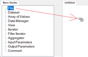
- Click Raster. The Select File(s) dialog appears.
-
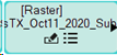
Navigate to the location where you saved the tutorial data machine_learning\supervised\training, click NAIP_DallasTX_Oct11_2020_Subset.tif, then click Open. A File node appears in the Untitled drawing area.
-
Click and drag another File node from the Basic Nodes list into the Untitled area of the ENVI Modeler. The Select Type dialog appears.
-
Click Regions of Interest. The Select File(s) dialog opens. Navigate to the location containing the tutorial data, machine_learning\supervised\training, click NAIP_DallasTX_Oct11_2020_Subset.xml, then click Open.
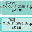
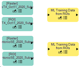
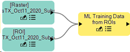
These two file nodes consist of a raster image and ROI labels. Both are needed to generate a single training raster during data prepration. You can organize the nodes in the Untitled node canvas as needed. To do this, click and drag a single node, or click in the empty Untitled draw area and drag the cursor over all nodes you intend to reposition. Selected nodes change to a lighter color, as illustrated above.
-
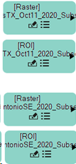
Repeat the two previous steps using the raster file NAIP_SanAntonioSE_2020_Subset.dat, and ROI file NAIP_SanAntonioSE_2020_Subset.xml. Both files are located in the tutorial data folder, machine_learning\supervised\training. When you are finished, you will have two raster file nodes and two ROI nodes.
Prepare the Data
To create training data for the supervised classifier, you must extract the labeled pixels using the raster and the associated ROIs. You will use the ENVI Machine Learning ML Training Data from ROIs task to create the training data. This task will extract all labeled pixels from the raster that are identified by the ROIs specified in the .xml file. A new raster containing a single row of spectra will be created. Dimensions of the training rasters are (rows=1, columns=input rasters columns, bands=input raster bands + 1). The additional band will provide a numeric value per pixel, this numeric value represent the class label value per pixel.
For this tutorial, we have the class labels Manmade, Trees, Ground, Water. These labels resolve to class values (0, 1, 2, 3). A pixel that was labeled Ground will be assigned a value of 2 in the label band, and so on for each pixel labeled.
-
In the ENVI Modeler Tasks Search field, type ML Training. Two tasks will appear.
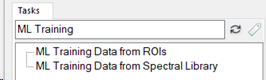
You will use ML Training Data from ROIs to generate training data. ML Training Data from Spectral Library is another Machine Learning data preparation task, which uses spectral libraries to collect pixel data for training.
-
Double-click on ML Training Data from ROIs, twice, to add two yellow nodes named "ML Training Data from ROIs" in the Untitled node canvas.
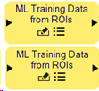
Arrange these nodes so they are paired to the right of the raster and ROI file nodes.
-
Click and drag the connector of the Raster node onto the ML Training Data from ROIs connector.
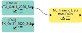
-
Click and drag the ROI node connector onto the ML Training Data from ROIs connector.
Be sure to pair the Raster and ROI nodes correctly when connecting to the ML Training Data from ROIs nodes:
|
Input Raster
|
NAIP_DallasTX_Oct11_2020_Subset.tif
|
|
Input ROI
|
NAIP_DallasTX_Oct11_2020_Subset.xml
|
|
|
|
|
Input Raster
|
NAIP_SanAntonioSE_2020_Subset.dat
|
|
Input ROI
|
NAIP_SanAntonioSE_2020_Subset.xml
|
-
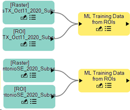
Repeat the previous two steps for the remaining Raster and ROI nodes. Once all nodes are connected, you should have the following.
-
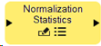
In the Tasks Search field, type Normalization Statistics. Double-click Normalization Statistics.
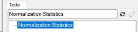
A new Normalization Statistics node appears on the untitled node canvas.
-
From the Basic Nodes list, double-click Aggregator. A new Aggregator node appears on the node canvas.

-
Click and drag both Raster node connectors onto the Aggregator connector.
-
Click and drag the Aggregator connector onto the Normalization Statistics connector.
-
Click and drag the Normalization Statistics connector onto both of the ML Training Data from ROIs node connectors.
After completing these steps, your node canvas should resemble the following image:
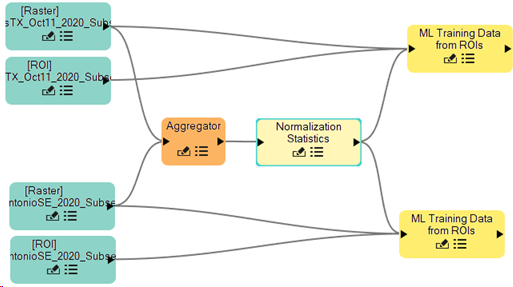
Normalization Statistics collects the minimum and maximum data values from an aggregate of input rasters. This is important during training, as the data will be scaled between 0 and 1 using the minimum and maximum values.
Connect to a Training Node
To train with the output data produced by ML Training Data from ROIs, you will need to aggregate the training data and connect it to a training task node. For this tutorial, we will use the Train Random Forest task, but you can select any of the supervised classification tasks. See ENVI Machine Learning Help for details.
-
In the Tasks Search field, type Train Random Forest. The Train Random Forest task appears.
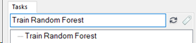
-
Double-click Train Random Forest. The node Train Random Forest appears on the node canvas.
-
From the Basic Nodes list, double-click Aggregator. A new Aggregator node appears on the node canvas.
-
Connect the ends of both ML Training Data from ROIs nodes to the Aggregator node connector.
-
Connect the end of the Aggregator node to the Train Random Forest node connector.
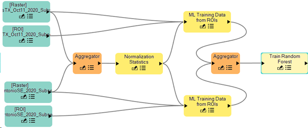
Your canvas should be similar to the image below.
Add Input Parameters
Input Parameters is a basic node that is reusable by many nodes. The Input Parameters node will be connected to multiple nodes on the canvas. By connecting input parameters, you are building a set of task inputs that can be specified when you run your model.
-
From the Basic Nodes list, double-click Input Parameters. An Input Parameters node appears on the node canvas.

-
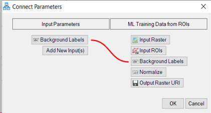
Connect the Input Parameters node to the beginning (left side) of one of the ML Training Data from ROIs nodes. The Connect Parameters dialog appears.
-
In the Connect Parameters dialog, click the Background Labels button under ML Training Data from ROIs. A red line connects Input Parameters [Add New Input(s)] to ML Training Data from ROIs [Background Labels]. Click OK.
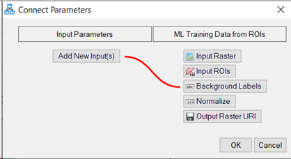
Repeat this step for the second ML Training Data from ROIs node. You should now have a [Background Labels] option under Input Parameters, click Input Parameters [Background Labels], then click OK.
-
Connect the Input Parameters node to the Train Random Forest node. The Connect Parameters dialog appears.
-
In the Connect Parameters dialog, under Train Random Forest, click Estimators, Balance Classes, Max Depth, and Output Model URI.
All four parameters are connected by colored lines to Input Parameters Add New Input(s). These are all parameters specific to the training task.
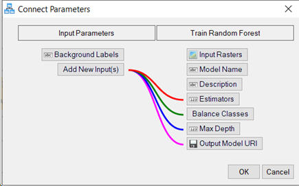
-
Click OK.
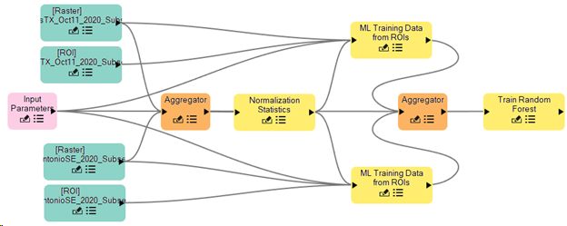
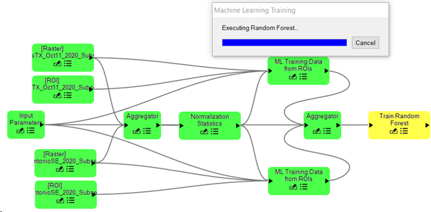
Your model should now resemble the following image, all connections are complete. Note the connection to the Train Random Forest node, from the Aggregator node, and the Input Parameters node are overlapping in the image below, there are two connections.
Run the Model
With the ENVI model complete, save your workflow and run it.
-
From the ENVI Modeler menu bar, select File > Save As. The Select Output Model File dialog appears. Specify the location to save the file and name it tutorial.model and click Save.
-
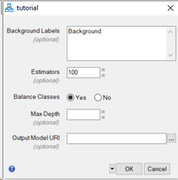
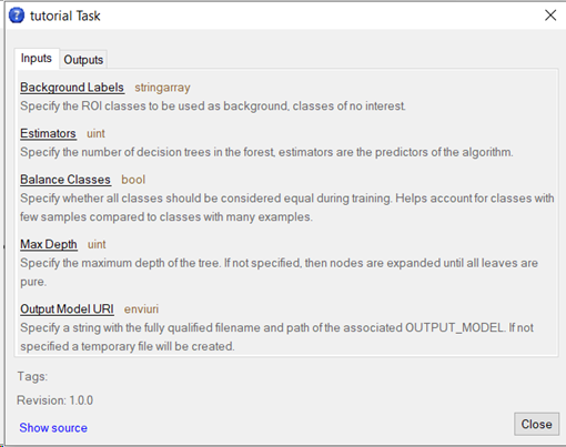
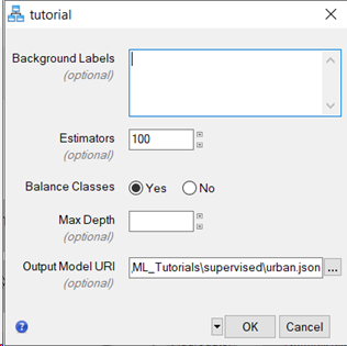
From the ENVI Modeler toolbar, click the Run button  . The tutorial task dialog appears with five task parameters.
-
You can get additional information about these parameters by clicking the Help  button in the lower left of the dialog. The tutorial Task help appears.
-
Click the Close button to dismiss the Help dialog.
-
In the Background Labels field, delete the text Background.
-
Leave the default values for the Estimators, Balance Classes, and Max Depth parameters.
- Click the Browse button
 next to Output Model URI. The Select Output Model URI dialog appears.
-
Select a file path and name the model urban.json, then click Open.
-
With all parameters set as specified, click the OK button. The ENVI Modeler nodes change colors to green showing completion of each step in the workflow. A Machine Learning Training progress dialog appears during the training step.
Training completes and nodes return to their original color scheme, the training progress dialog closes.
-
Close the ENVI Modeler dialog.
Perform Classification
Now that the trained supervised classification model created, you can run the classification process. You will use the Machine Learning Classification tool in the ENVI Toolbox for these steps.
-
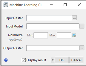
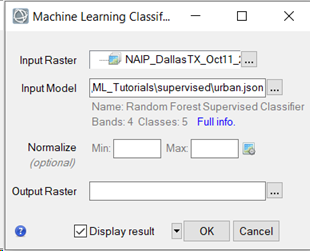
In the ENVI Toolbox, expand the Machine Learning folder and double-click Machine Learning Classification. The Machine Learning Classification dialog appears.
-
Click the Browse button next to Input Raster. The Data Selection dialog appears.
-
Click the Open File button  in the bottom left of the Data Selection dialog. The Open dialog appears.
-
Go to the location were you saved the tutorial data and select machine_learning\supervised\classification/NAIP_DallasTX_Oct11_2020.tif, then click Open.
-
Click OK.
-
Click the Browse button next to Input Model. The Please Select a File dialog appears.
-
Go to the location were you saved the model urban.json. Select it and click Open.
-
Leave the Normalize fields empty, the minimum and maximum values will be used from the model file.
-
Leave the Output Raster field blank. A temporary file will be created.
-
Enable Display result if is not already selected, and click OK. Classification starts and the Machine Learning Classification progress dialog appears.
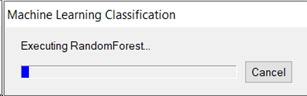
Classification completes after 1 to 2 minutes, time will depend on the system.
-
The classification raster displays in the ENVI view. The Layer Manager shows the classes Unclassified, Water, Ground, Trees, and Manmade. The class Unclassified was not used during the labeling process; this class represents any unclassified pixels if present. The colors used for each label during the labeling process are also the colors used to identify targets in the classification result.
-
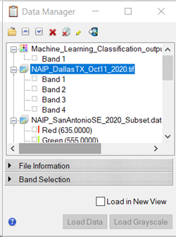
From the ENVI toolbar, click the Data Manager button  . The Data Manager dialog appears.
-
Right-click NAIP_DallasTX_Oct11_2020.tif and click Load Default. The original image is displayed in the ENVI view, the Layer Manager places the raster above the classification raster.
-
In the Layer Manager, click and drag the Machine_Learning_Classification_output* raster above the raster NAIP_DallasTX_Oct11_2020.tif.
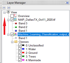
The ENVI view updates with the classification raster displaying over the original image.
-
From the ENVI toolbar, move the Transparency slider back and forth to explore the classification result compared to the original image. You will notice the model did a pretty good job identifying the correct classes, but it is not perfect. Shadows throughout the image have been classified as Manmade. One way to try and eliminate this would be to create a Shadows class, or collect shadows as part of the Background class.
Another imperfection is that the football stadium is partially labeled as water. This could be mitigated by adding labeled examples of the stadium and retraining the model. Enter the pixel coordinates 7784p,7148p in the Go To field and press Enter to jump to the stadium.
-
Optionally, run through the classification workflow again to see how well your model does with the additional classification scene. The image can be found in the tutorial data machine_learning\supervised\classification\NAIP_SanAntonioSE_2020.dat.
-
When you are finished, exit ENVI.
Final Comments
In this tutorial you learned how to model a custom Machine Learning workflow to train a Random Forest classifier using labeled data. You learned it’s possible to train a model using multiple rasters and multiple labels and generate good results.
In conclusion, machine learning technology provides a robust solution for learning complex spectral patterns in data, meaning that it can extract features from a complex background, regardless of their shape, color, size, and other attributes.
For more information about the capabilities presented here, and other machine learning offerings, refer to the ENVI Machine Learning Help.