In this tutorial you will use ENVI Deep Learning to create a classification image showing different types of property damage from a tornado. You will learn how to use regions of interest (ROIs) to label different features in imagery and how to train a TensorFlow deep learning model to learn those features in a separate but similar image. The tutorial can be used with ENVI Deep Learning 2.1 or later.

See the following sections:

• System Requirements
• Files Used in This Tutorial
• Background
• Label Training Rasters With ROIs
• Train a Deep Learning Model
• Perform Classification
• Final Comments
• References

System Requirements

Refer to the Systems Requirements topic.

Files Used in This Tutorial

Sample data files are available on our ENVI Tutorials web page. Click the "Deep Learning" link in the ENVI Tutorial Data section to download a .zip file containing the data. Extract the contents to a local directory.

The files for this tutorial are in the tornado directory.

ImageToClassify.dat

TrainingRaster1.dat

TrainingRaster2.dat

TrainingRaster3.dat

TrainingRaster4.dat

TrainingRaster1ROIs.xml

TrainingRaster2ROIs.xml

TrainingRaster3ROIs.xml

TrainingRaster4ROIs.xml

TrainedModel.h5

Background

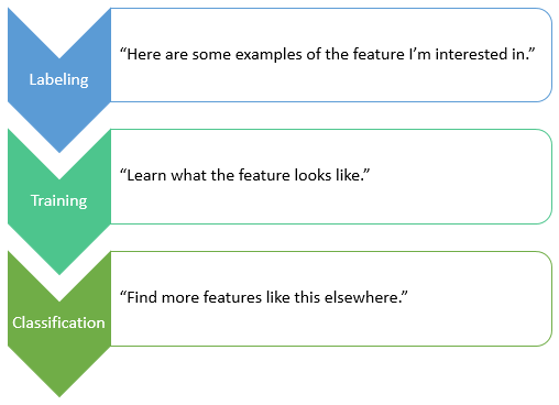
A common use of deep learning in remote sensing is pixel-based feature extraction; that is, identifying specific features in imagery such as vehicles, road centerlines, or utility equipment. Through a process called labeling, you mark the locations of features in one or more images. With training, you pass the labeled data to a deep learning model so that it learns what the features look like. Finally, the trained model can be used to look for more of the features in the same image or other images with similar properties. This is the classification step.

You can train the deep learning model to find all instances of the features (for example, conducting an inventory of assets) or to draw approximate boundaries around the features.

In this tutorial, you will train a deep learning model to look for different levels of structural damage from an EF-5 tornado in Joplin, Missouri, USA that occurred on 22 May 2011. The tornado killed 158 people and caused damages that totalled $2.8 billion, making it the costliest tornado in U.S. history. According to the National Weather Service, nearly 7,000 homes were completely destroyed and 875 homes suffered minor to severe damage.

Aerial images captured after natural disasters like this can reveal the extent of property damage and changes to the landscape. Visually inspecting images and marking locations where damage occurred can take a significant amount of time for an analyst, especially if the damage covers a large geographic area. This can further delay the time it takes to issue insurance payouts so that rebuilding can begin. Machine learning can be used to quickly identify areas from imagery that suffered various levels of property damage, which can help inspectors determine specific locations to focus on in the field.

Deep learning is a more sophisticated form of machine learning that can excel in scenarios like this, where the distinction between damaged roofs and structural deterioration can be confusing in aerial imagery. ENVI Deep Learning uses TensorFlow technology, which is based on a convolutional neural network (CNN). It looks for spatial and spectral patterns in image pixels that match the training data it was provided. Specifically, this tutorial uses the pixel segmentation approach to training.

The first step in training a deep learning model is to collect samples of features that you want the model to find—a process called labeling. In this tutorial, you will train a deep learning model to look for different indicators of structural damage, which will result in a classification image with multiple classes.

Label Training Rasters With ROIs

To begin the labeling process, you need at least one input image from which to collect samples of the features you are interested in. These are called training rasters. They can be different sizes, but they must have consistent spectral and spatial properties. Then you can label the training rasters using regions of interest (ROIs). The easiest way to label your training rasters is to use the Deep Learning Labeling Tool. Follow these steps:

1. Start ENVI.
2. In the ENVI Toolbox, select Deep Learning > Deep Learning Guide Map. The Deep Learning Guide Map provides a step-by-step approach to working with ENVI Deep Learning. It guides you through the steps needed for labeling, training, and classification.
3. Click the following button sequence: Pixel Segmentation > Train a New Pixel Model > Label Rasters. The Labeling Tool appears.
4. Keep the Deep Learning Guide Map open because you will use it later in the tutorial.

Set Up a Deep Learning Project

Projects help you organize all of the files associated with the labeling process, including training rasters and ROIs. They also keep track of class names and the values you specify for training parameters.

1. Go to the directory where you saved the tutorial files, and create a subfolder called Project Files.
2. Select File > New Project from the Labeling Tool menu bar. The Create New Labeling Project dialog appears.
3. In the Project Name field, enter Tornado Damage.
4. Click the Browse button next to Project Folder and select the Project Files directory you created in Step 1.
5. Click OK.

When you create a new project and define your training rasters, ENVI creates subfolders for each training raster that you select as input. Each subfolder will contain the ROIs and label rasters created during the labeling process.

The next step is to define the classes you will use.

Define Classes

Use the Class Definitions section of the Labeling Tool to define the features you will label. The feature names determine the class names in the output classification image.

1. Click the Add button in the lower-left corner of the Class Definitions section.
2. In the Name field, type Roof Damage, then click the button. The feature is added to the Class Definitions list.
3. Click in the color box next to Roof Damage, and change it to a yellow color.
4. Click the Add button to add another feature.
5. In the Name field, type Structural Damage, then click the button.
6. Click in the color box next to Structural Damage, and change it to an orange color.
7. Click the Add button .
8. In the Name field, type Rubble, then click the button.
9. Click in the color box next to Rubble, and change it to a red color.
10. Click the Add button .
11. In the Name field, type Blue Tarps, then click the button.
12. Click in the color box next to Blue Tarps, and change it to a blue color.

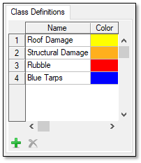
The Class Definitions list should look similar to this:

Next, you will select the rasters that you want to train.

Add Training Rasters

1. Click the Add button below the Rasters section of the Labeling Tool. The Data Selection dialog appears.
2. Click the Open File button at the bottom of the Data Selection dialog.
3. Go to the directory where you saved the tutorial data. Use the Ctrl or Shift key to select the following files, then click Open.
   • TrainingRaster1.dat
   • TrainingRaster2.dat
   • TrainingRaster3.dat
   • TrainingRaster4.dat
4. Click the Select All button in the Data Selection dialog, then click OK.

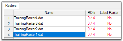
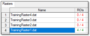
   The training rasters are added to the Rasters section of the Deep Learning Labeling Tool. The table in this section has two additional columns: "ROIs" and "Label Raster." Each "ROIs" table cell shows a red-colored fraction: 0/4. Each training raster has four associated ROIs because you specified four classes. The "0" means that none of the four ROIs has been drawn yet. The "Label Raster" column shows a red-colored "No" indicating that no label rasters have been created yet.

   

Now you are ready to label the features in your training rasters by drawing ROIs in them.

Draw and Restore ROIs

For the first part of this exercise, you will learn how to draw polygon ROIs around examples of structures that have varying levels of damage. The labeling process often takes the most amount of time in any deep learning project. It can take several hours, or even days, depending on the size of the images and the number of features. To save time in the second part of the exercise, you will import ROIs that were already created for you.

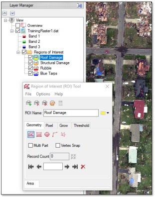
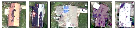
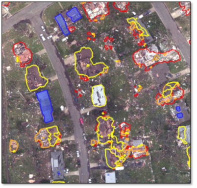
1. Select TrainingRaster1.dat and click the Draw button . The training raster is displayed in the Image window. ENVI creates a new set of ROIs with the same names and colors as the classes that you defined. The ROIs are listed in the Layer Manager and Data Manager. The Region of Interest (ROI) Tool appears, with the "Roof Damage" ROI selected. The following image shows an example. The cursor changes to a crosshair so that you can begin drawing ROI polygons.

   

   Note: If you do not want to learn to draw ROIs, you can skip Steps 2-6 and instead restore ROIs that were created for you. To do this, click the Options button and select Import ROIs. Select the file TrainingRaster1ROIs.xml, match the class names to the ROI names, and click OK. The ROIs will display in the Image window.

2. For the Roof Damage class and ROI, click to draw polygons around entire roofs that are missing shingles or otherwise showing signs of minor damage; for example:



To complete the last segment of the polygon, either double-click or right-click and select Complete and Accept Polygon. Here are some additional tips for drawing ROIs:

• To remove the last segment drawn, click the Backspace key on your keyboard.
• To cancel drawing a polygon, right-click and select Clear Polygon.
• If your mouse has a middle button, click and drag it to pan around the display. If it has a scroll wheel, use that to zoom in and out of the display. These actions allow you to move around the image without disrupting the ROI drawing process.
• If you click the Pan, Select, or Zoom tools in the toolbar, the ROI Tool will lose focus. If this happens, double-click the Roof Damage ROI in the Layer Manager to resume drawing records for that ROI.
• To delete a polygon record that has already been drawn, click the Goto Previous Record button in the Region of Interest (ROI) Tool until that record is centered in the display. Then click the Delete Record button.
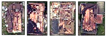
3. To select examples of the next class, double-click the Structural Damage ROI in the Layer Manager. The ROI Tool updates to show this ROI. Locate partial or entire buildings that are still intact but are missing roofs and exposing the underlying lumber framing. These buildings likely have major structural damage; for example:



Already you can see that it is difficult to clearly separate the first two classes. Some buildings have a combination of roof and structural damage; for example:



In these cases, draw polgyons for Roof Damage around the part of the building that is missing shingles. Then switch to the Structural Damage ROI and draw polygons around the areas indicating structural damage on the same building; for example:



The polygons do not have to be exact when the boundaries between classes are indistinct.

4. Double-click the Rubble ROI in the Layer Manager. The ROI Tool updates to show this ROI. Draw polygons around areas where structures have been completely destroyed, leaving behind piles of rubble; for example:



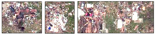
Often there is no clear boundary between rubble and the surrounding landscape, so draw the polygons around their approximate locations; for example:



5. Double-click the Blue Tarp ROI in the Layer Manager. The ROI Tool updates to show this ROI. Draw polygons along the boundaries of blue-colored tarps on roofs. Homeowners often place tarps on sections of roofs that have been exposed from the tornado so that subsequent rainfall will not further damage their homes; for example:



6. Continue drawing ROIs for each class on every example in TrainingRaster1.dat. It is important to identify as many examples as possible to train the deep learning model. When you double-click ROIs in the Layer Manager to select them, the "ROIs" column updates in the Deep Learning Labeling Tool to show the fraction of ROIs drawn to the total number of ROIs. The text changes to green; for example:



7. When you are finished drawing ROIs, select TrainingRaster2.dat in the Labeling Tool and click the Draw button. This training raster is displayed in the Image window. ENVI automatically saves the ROIs that you drew for the last training raster, so you do not have to worry about losing your progress. The ROIs are saved to a file named rois.xml in a TrainingRaster1_dat_* subdirectory under Project Files.
8. For the remaining part of this exercise, you will restore an existing set of ROIs instead of manually drawing them. Click the Options button in the Deep Learning Labeling Tool and select Import ROIs. The Select ROIs Filename dialog appears.
9. Go to the directory where you saved the tutorial files and select TrainingRaster2ROIs.xml. Click Open. The Match Input ROIs to Class Definitions dialog appears.
10. Click the Roof Damage button under Input ROIs, then click the same button on the right side under Class Definitions. A line is drawn between the two.
11. Repeat this step with the other ROIs and classes, then click OK.



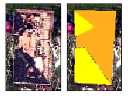
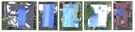
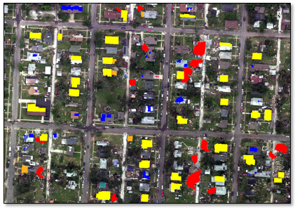
The second training raster and ROIs are displayed in the Image window:



These ROIs were a best attempt to identify examples that represented all of the classes, given that class boundaries are not always clearly defined.

12. Uncheck the individual ROIs in the Layer Manager to see the underlying pixels in the image.
13. You can optionally add or remove individual ROI records from this training raster; however, it is not required for this tutorial. If you do this, do not select File > Save As in the ROI Tool to save your changes as this can lead to issues with the current project. You do not have to take any action; the changes will automatically save when you select a different training raster.
14. Select TrainingRaster3.dat in the Labeling Tool and click the Draw button.
15. Click the Options button in the Labeling Tool and select Import ROIs. The Select ROIs Filename dialog appears.
16. Select the file TrainingRaster3ROIs.xml and click Open. The Match Input ROIs to Class Definitions dialog appears.
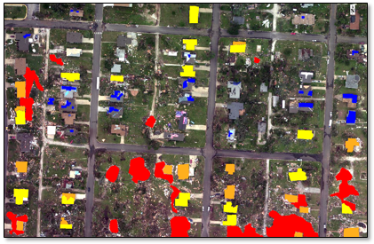
17. Match the ROI names with the class names and click OK. The third training raster and ROIs are displayed in the Image window:



18. Select TrainingRaster4.dat in the Labeling Tool and click the Draw button.
19. Click the Options button in the Labeling Tool and select Import ROIs. The Select ROIs Filename dialog appears.
20. Select the file TrainingRaster4ROIs.xml and click Open. The Match Input ROIs to Class Definitions dialog appears.
21. Match the ROI names with the class names and click OK. The fourth training raster and ROIs are displayed in the Image window:

View Project and Labeling Statistics

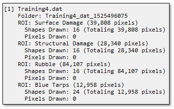
1. Click the Options drop-down list and select Show Labeling Statistics to view information about the current project and how much labeling was performed; for example:



2. Close the Project Statistics dialog.

Once you have labeled all of your training rasters with ROIs, the next step is to train the deep learning model.

Train the Deep Learning Model

Training involves repeatedly exposing label rasters to a model. Over time, the model will learn to translate the spectral and spatial information in the label rasters into a classification image that maps the features it was shown during training.

1. From the Train drop-down list at the bottom of the Labeling Tool, select Pixel Segmentation. The Train Deep Learning Pixel Segmentation Model dialog appears.

2. The Model Architecture parameter specifies the type of network to train the model with. Given the inconsistent appearance of damage types for this tutorial, SegUNet is recommended. From the Model Architecture drop-down list, select SegUNet. SegUNet++ is better suited for well-defined, consistent features.

3. The Patch Size parameter is the number of pixels along one side of a square "patch" that will be used for training. Keep the default value of 464.
4. The Training/Validation Split (%) slider specifies what percentage of data to use for training versus testing and validation. Keep the default value of 80%.
5. Disable the Shuffle Rasters option.
6. The following parameters are advanced settings for users who want more control over the training process. For this tutorial, use the following values:
   • Number of Epochs: 20
   • Number of Patches per Image: 100
   • Solid Distance: 0 for all classes
   • Blur Distance: Click the Set all to same value button . Enter 1 to 8 and click OK.
   • Class Weight: Min 0, Max 3
   • Loss Weight: 0.5
7. In the Output Model field, choose an output folder and name the model file TrainedModel.h5, then click Open. This will be the "best" trained model, which is the model from the epoch with the lowest validation loss.
8. In the Output Last Model field, choose an output folder and name the model file TrainedModelLast.h5, then click Open. This will be the trained model from the last epoch.
9. Click OK. In the Labeling Tool, the Label Raster column updates with "OK" for all training rasters, indicating that ENVI has automatically created label rasters for training.

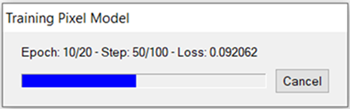
As training begins, a Training Model dialog reports the current Epoch, step, and training loss, for example:

Also, A TensorBoard page displays in a new web browser. This is described next, in View Training and Accuracy Metrics.

Training a model takes a significant amount of time due to the computations involved. Processing can take several minutes to a half-hour to complete, depending on your system hardware and GPU. If you do not want to wait that long, you can cancel the training step now and use a trained model (TrainedModel.h5) that was created for you, later in the classification step. This file is included with the tutorial data.

View Training and Accuracy Metrics

TensorBoard is a visualization toolkit included with TensorFlow. It reports real-time metrics such as Loss, Accuracy, Precision, and Recall during training. Refer to the TensorBoard online documentation for details on how to use it.

Follow these steps:

1. Set the Smoothing value on the left side of the TensorBoard to 0.999. This will allow you to visualize the lines for batch, train, and validation more clearly. Smoothing is a visual tool to help see the entire training session briefly and provide insight into model convergence. Setting smoothing to 0.0 will provide normal values for the given step of a batch for the given epoch.

2. After the first few epochs are complete, TensorBoard provides data for the training session. Several metrics provide insight to how the model is conforming to the data. Scalar metrics include overall, and individual class accuracy, precision, and recall. To start, click on Loss in TensorBoard to expand and view a plot of training and validation loss values. Loss is a unitless number that indicates how closely the classifier fits the validation and training data. A value of 0 represents a perfect fit. The farther the value from 0, the worse the fit. Loss plots are provided per batch and per step. Ideally, the training loss values reported in the train loss plot should decrease rapidly during the first few epochs, then converge toward 0 as the number of epochs increases. The following image shows a sample loss plot during a training session of 20 epochs. Your plot might look different:

   

   It is normal to see spikes in Loss values during training. Moving the cursor from left to right in the plot will show different values per step. Batch steps are listed along the X-axis, beginning with 0. A step is calculated with the following equation, (nSteps * nEpochs) * Batch Size. For this tutorial nSteps is 100 steps per epoch, epochs are 20, and Batch Size is 3. (100 * 20) * 3 evaluates to 6,000 total training steps. In the gray section of the image above, the Step column shows 6k for train and validation.

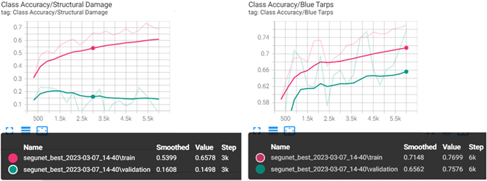
3. In the loss plot in the step above, notice the divergence of the validation line (green), versus train (pink), and batch (blue). This can be due to several factors, the most obvious factor comes from viewing the individual class accuracy metrics and confusion matrices. In the TensorBoard dashboard, select SCALARS, then click Class Accuracy to expand the accuracy plots for each class. Below are the two extremes: the worst class accuracy, Structural Damage on the left, and best class accuracy, Blue Tarps on the right. The train and validation values for class Structural Damage are moving in the opposite direction. Blue Tarps train and validation values are in sync, looking at the confusion matrix can help show why this is occurring.

   

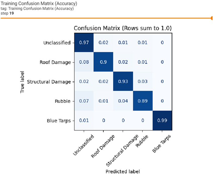
4. In the TensorBoard dashboard, select IMAGES. From this menu, can view a confusion matrix for the training dataset and the validation dataset. A confusion matrix is a matrix of information that tells you where a model is confused. The confusion matrix provides a true label to a predicted label, showing the prediction for the various classes between 0 and 1. All rows add up to 1. As the image in the next step shows, the true label is on the left along the Y axis. The Predicted labels are shown at the bottom along the X axis. The ideal scenario would be for all classes to show a value of 1 in the predicted columns for each label.

5. Click on the Training Confusion Matrix image to make it larger. The Training Confusion Matrix is based on how well the model predicted labeled data used during training. From a training data perspective, the dark blue diagonal, top left through the center to the bottom right is good. This shows that the training data provided was sufficient for the model to converge on all classes.

   

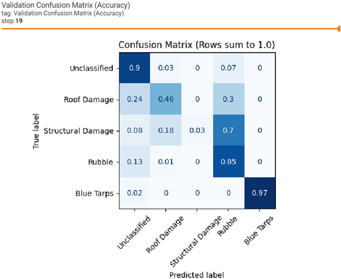
6. Click on the Validation Confusion Matrix image to make it larger. The Validation Confusion Matrix is based on how well the model predicted labels not used during training. Although validation data is provided to the model during training, it is only used for comparison at the end of each epoch to calculate the epochs error. The error is indicated by the loss score throughout training. The image below is much different than the training confusion matrix. It indicates several possible issues with the data or data distribution. It is possible the distribution of validation data was limited for examples containing Roof Damage labels, and more so for Structural Damage labels. Class Roof Damage is confused with background data and Rubble. While class Structural Damage is confused with Rubble and Roof Damage.

   

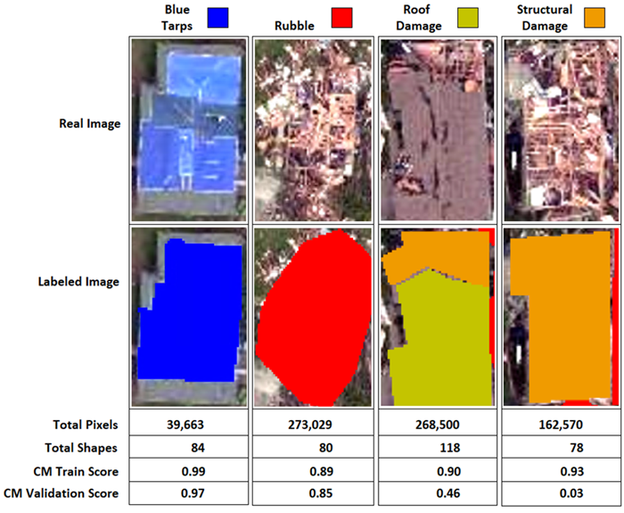
   Given the type of features to learn, even for a person, it could be difficult to differentiate Structural Damage from Rubble. The next image shows a side-by-side comparison of each label type, total pixels, total labels, and the final epochs train and validation confusion matrix scores.

   

   Training Deep Learning models, especially with complicated data will usually require trial and error. Retraining the model in this tutorial will likely produce a different set of results and statistics every time. There is no perfect answer for creating good models, but an educated assessment goes along way for improving a model.

   Some observations looking at the image above and the CM Validation Score:

   • Blue Tarps scored the highest out of all classes and has the least amount of training data. You could speculate that Blue Tarps compared to the other classes is a much simpler feature to learn, and unique in color compared to the others.

   • Rubble was the second highest scoring class per validation, and arguably many features in the training labels look very similar to Rubble. Additionally, Rubble labels offer the highest number of pixels used during training.

   • Roof Damage was the third highest scoring class per the validation score. Roof Damage scored a 0.24 as Unclassified, and 0.30 as Rubble, with an actual label score of 0.46. Roof tops in general have a similar look as parking lots and roadways which could explain the unclassified error. Roof Damage is almost always mixed closely with Rubble and Structural Damage and may simply need many more labeled examples for training and validation.

   • Structural Damage scored much higher in the training confusion matrix at 0.93 and scored very low in the validation confusion matrix at 0.03. There are likely several reasons why validation performed so poorly. Lack of data, Structural Damage provided the second to last least number of pixels, and the least number of labeled shapes overall. Based on the 80/20 training and validation data split, only 15-16 examples would have been provided for validation while training received 62-63 examples. This class is one of the most complicated features out of the four classes, if not the hardest to learn and the data shows that. Providing more examples and clean labels might reduce model confusion.

7. The full breadth of all metrics is beyond the scope of this tutorial. You can explore the other metrics not covered in this tutorial. See the menu options SCALARS, DISTRIBUTIONS, HISTOGRAMS, and TIME SERIES. When you are finished evaluating training and accuracy metrics:

   • Close the TensorBoard page in your web browser.
   • Close the Deep Learning Labeling Tool. All files and ROIs associated with the "Tornado Damage" project are saved to the Project Files directory when you close the tool.
   • Close the ROI Tool.
   • Click the Data Manager button in the ENVI Toolbar. In the Data Manager, click the Close All Files button .

Perform Classification

Now that you have a model that was trained to find examples of property damage in four training rasters, you will use the same model to find similar instances in a different aerial image of Joplin. This is one of the benefits of ENVI Deep Learning; you can train a model once and apply it multiple times to other images that are spatially and spectrally similar.

1. Click the Open button in the Data Manager.
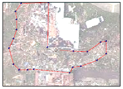
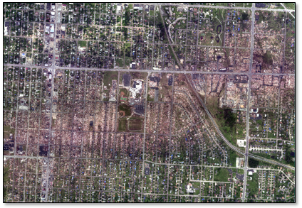
2. Go to the location where you saved the tutorial data and select the file ImageToClassify.dat. The image appears in the display.
3. Press the F12 key on your keyboard to zoom out to the full extent of the image. This is a different image of the city of Joplin, acquired from the same sensor and on the same day. It is much larger than the training rasters (10,400 by 7,144 pixels). The path of the tornado is visible as a lighter shade through the middle of the image. You will use the trained model to classify this image.



4. In the Deep Learning Guide Map, click the Classify Raster Using a Trained Model button. The TensorFlow Pixel Classification dialog appears.
5. The Input Raster field is already populated with ImageToClassify.dat. You do not need to change anything here.
6. In the Input Model field, use one of the following options for selecting a model file:
   • Select the file TrainedModel.h5 that you just created during the training step.
   • If you chose to cancel the training process and want to use a trained model that was already created for you, go to the location where you saved the tutorial and select the file TrainedModel.h5.
7. In the Output Classification Raster field, choose a location for the output classification raster. Name the file TornadoClassification.dat.
8. Enable the Display result option for Output Classification Raster.
9. In the Output Class Activation Raster field, choose a location for the output class activation raster. Name the file TornadoClassActivation.dat.
10. Disable the Display result option for Output Class Activation Raster. You will display the individual bands of this raster later in the tutorial.

11. Click OK. A Classifying Raster progress dialog shows the status of processing:

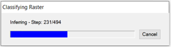
When processing is complete, the classification result is displayed in the Image window; for example:

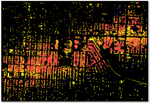
Your result may be slightly different than what is shown here. Training a deep learning model involves a number of stochastic processes that contain a certain degree of randomness. This means you will never get exactly the same result from multiple training runs.

1. Click the Zoom drop-down list in the ENVI toolbar and select 100% (1:1).
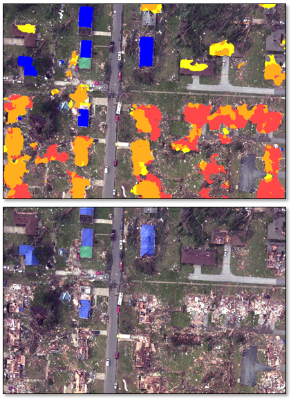
2. Uncheck the Unclassified class in the Layer Manager. The individual classes are displayed over the true-color image (ImageToClassify.dat).
3. Toggle the TornadoClassification.dat layer on and off in the Layer Manager to view the underlying pixels in the true-color image. The following example shows a comparison between the two layers:

Optional: Export Classes to Shapefiles

Now that you have created a classification image, you may want to create shapefiles of the classes for further GIS analysis or presentations. Follow these steps:

1. Type vector in the search window of the ENVI Toolbox.
2. Double-click the Classification to Vector tool in the search results. The Data Selection dialog appears.
3. Select TornadoClassification.dat and click OK. The Convert Classification to Vector Shapefile dialog appears.
4. Select all of the classes listed in the Export Classes field, except for Unclassified.
5. From the Output Method drop-down list, select One Vector Layer Per Class. This will create separate shapefiles for each class.
6. Click the No radio button next to Apply Symbology.
7. In the Output Vector field, keep the default root name of ClassificationToShapefile.shp. ENVI will append the class names to this root name.
8. Click OK. ENVI creates the shapefiles but does not display them.
9. Uncheck the TornadoClassification.dat layer in the Layer Manager to hide it.
10. Click the Open button in the ENVI toolbar. A file selection dialog appears.
11. Go to the directory where you saved the shapefiles. Use the Ctrl or Shift key to select the following files, then click Open:
    • ClassificationToShapefile_Blue_Tarp.shp
    • ClassificationToShapefile_Roof_Damage.shp
    • ClassificationToShapefile_Rubble.shp
    • ClassificationToShapefile_Structural_Damage.shp

    The shapefiles are displayed over the true-color image (ImageToClassify.dat) and are listed in the Layer Manager. The default colors are different than those of the classes and ROIs. You will change the colors in the next step.

12. Double-click ClassificationToShapefile_Blue_Tarp.shp in the Layer Manager. The Vector Properties dialog appears.
13. On the right side of the Vector Properties dialog, click inside of the Line Color field under Shared Properties. A drop-down arrow appears. Click on this and change the color to blue (0,0,240).
14. Click inside of the Line Thickness field under Shared Properties. A drop-down arrow appears. Click on this and select a line thickness of 3.
15. Click the Apply button.
16. When you change the properties of a shapefile, or any other vector format, they only persist in the current ENVI session. To avoid having to reapply the properties of the shapefile each time you start ENVI, you can save the property symbology to a file on disk. When ENVI reads and displays the shapefile, it will automatically apply the symbology. To save the symbology for this shapefile, click the Symbology drop-down list and select Save/Update Symbology File. ENVI creates a file called ClassificationToShapefile_Blue_Tarp.evs in the same directory as the shapefiles.
17. Click OK in the Vector Properties dialog.
18. Repeat Steps 12-17 for the remaining shapefiles, using the colors and line thickness below:

Shapefile	Line Color	Line Thickness
ClassificationToShapefile_Roof_Damage.shp	Yellow (255,255,29)	3
ClassificationToShapefile_Rubble.shp	Red (240,240,0)	3
ClassificationToShapefile_Structural_Damage.shp	Orange (255,175,29)	3

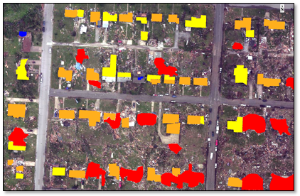
The following image shows an example of the colored shapefiles displayed over the true-color image. Your results will be different:

View Class Activation Rasters

Another output of the classification process is a series of class activation rasters. Earlier in the TensorFlow Pixel Classification tool, you created a file named JoplinClassActivation.dat. Each band of this file contains a grayscale class activation raster whose pixels indicate the probability of belonging to a specific feature. In this case, it has five bands: Unclassified, Blue Tarp, Roof Damage, Rubble, and Structural Damage. Follow these steps to view the class activation rasters:

1. Right-click on each shapefile in the Layer Manager and select Remove. The only image that should be displayed is ImageToClassify.dat.
2. Open the Data Manager and look for JoplinClassActivation.dat. Expand the filename to see the individual bands, if needed.
3. Select the Roof Damage band and click the Load Grayscale button. The class activation raster for that class is displayed in the Image window.
4. At the bottom of the ENVI application is the Status bar. Right-click in the middle segment of the Status bar and select Raster Data Values. As you move your cursor around the class activation raster, its pixel values are displayed in the Status bar; for example:



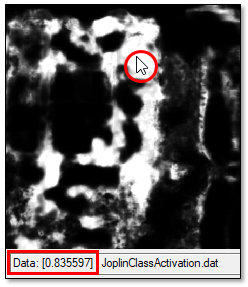
The pixel values range from 0 to 1.0. Higher values (bright pixels) represent high probabilities of belonging to the Roof Damage class.

Apply a Raster Color Slice to the Class Activation Raster

To better visualize the class activation raster, you can apply a raster color slice to it. A color slice divides the pixel values of an image into discrete ranges with different colors for each range. Then you can view only the ranges of data you are interested in.

1. In the Layer Manager, right-click on JoplinClassActivation.dat and select New Raster Color Slice. The Data Selection dialog appears.
2. Select Roof Damage under JoplinClassActivation.dat and click OK. The Edit Raster Color Slices dialog appears. The pixel values are divided into equal increments, each with a different color.



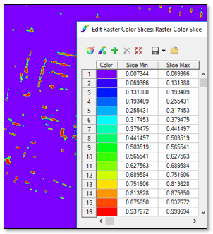
3. Click OK in the Edit Raster Color Slices dialog to accept the default categories and colors.
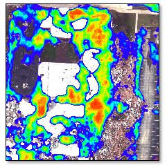
4. In the Layer Manager, uncheck the JoplinClassActivation.dat layer to hide it.
5. In the Raster Color Slice layer in the Layer Manager, uncheck the purple color slice range. This is the background. The remaining colors (blue to red) identify pixels with increasing probabilities of matching "Roof Damage," according to the training data you provided. The following image shows an example:



6. Repeat these steps with the remaining class activation rasters.

Final Comments

In this tutorial you learned how to use ENVI Deep Learning to extract multiple features from imagery using polygon ROIs to label the features. ROIs provide a quick and efficient way to identify all instances of a certain feature in your training images. Once you determine the best parameters to train a deep learning model, you only need to train the model once. Then you can use the trained model to extract the same feature in other, similar images.

For further experimentation, consider running the ENVI Modeler model file named Deep_Learning_Randomize_Training.model. This model is provided with the ENVI Deep Learning installation. This ENVI Modeler model performs a full, automated ENVI Deep Learning workflow multiple times, each with a different set of randomized training parameters. Each result is displayed separately so that you can decide which training run produced the best TensorFlow model. For more information, see Randomize Training Parameters.

In conclusion, deep learning technology provides a robust solution for learning complex spatial and spectral patterns in data, meaning that it can extract features from a complex background, regardless of their shape, color, size, and other attributes.

For more information about the capabilities presented here, please refer to the ENVI Deep Learning Help.

References

National Weather Service. "7th Anniversary of the Joplin Tornado - May 22, 2011." https://www.weather.gov/sgf/news_events_2011may22 (accessed 29 August 2019).