In this tutorial you will use ENVI Deep Learning to train an object detection model to find a specific feature in an aerial image. You will learn how to use annotations to label examples of the feature and how to train a deep learning model to learn that feature in a separate but similar image. The tutorial workflow is compatible with ENVI Deep Learning version 4.0 and higher.
This tutorial requires a separate installation and license for ENVI Deep Learning; contact your sales representative for more information.
See the following sections:
System Requirements
Refer to the System Requirements topic.
Files Used in This Tutorial
Sample data files are available on our ENVI Tutorials web page. Click the Deep Learning link in the ENVI Tutorial Data section to download a .zip file containing the data. Extract the contents of the .zip file to a local directory. The files for this tutorial are located in the object_detection folder.
The three images used in the tutorial are spatial subsets of orthorectified aerial images provided by the Denver Regional Council of Governments (DRCOG) Regional Data Catalog (https://data.drcog.org). Images are in the public domain. License terms are governed by CC BY 3.0 (http://creativecommons.org/licenses/by/3.0).
The images have three bands (red/green/blue) with a spatial resolution of 0.4921 U.S. Survey Feet.
|
File |
Description |
|
DRCOG_AerialImage1.dat
|
DRCOG image (3,490 x 5,458 pixels) used for training
|
|
DRCOG_AerialImage2.dat
|
DRCOG image (10,000 x 3.080 pixels) used for validation
|
|
ImageToClassify.dat
|
DRCOG image (10,000 x 10,000 pixels) used for classification
|
|
Handicap_Parking_Spots1.anz
|
Rectangle annotation labels of handicap parking spots in DRCOG_AerialImage1.dat
|
|
Handicap_Parking_Spots2.anz
|
Rectangle annotation labels of handicap parking spots in DRCOG_AerialImage2.dat
|
Background
Object detection can be used to extract objects that touch or overlap, unlike pixel segmentation. ENVI now uses the RT-DETR (Real-Time Detection Transformer) architecture for object detection based on the original RT-DETR model introduced by Zhao et al. (2023). The following reference is the basis for that algorithm:
Reference: Yian Zhao, Wenyu Lv, Shangliang Xu, Jinman Wei, Guanzhong Wang, Qingqing Dang, Yi Liu, Jie Chen. [2304.08069] DETRs Beat YOLOs on Real-time Object Detection.
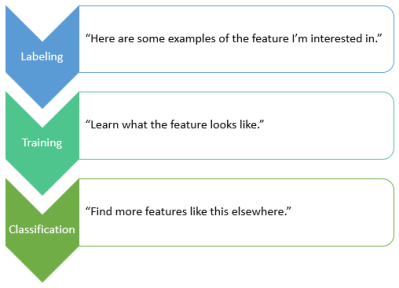
You pass labeled data to an object detection model so that it learns what the feature looks like. This is the training process. The trained model can be used to look for more of the same feature in the same image or other images with similar properties. This is the classification process.
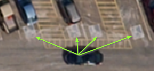
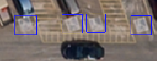
In this tutorial, you will train an object detection model to find parking spots with handicap signs painted on the pavement; for example:
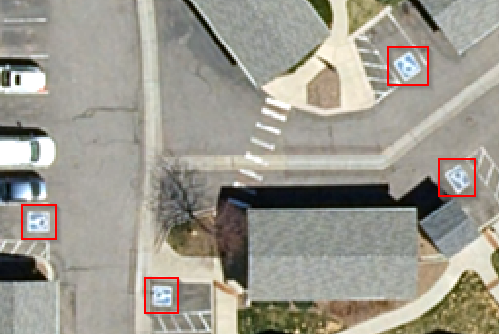
It simulates a workflow where urban planners or traffic engineers can locate road markings, fire hydrants, manhole covers, or related features, in high-resolution aerial imagery.
Label Training Rasters with Annotations
To begin the labeling process, you need at least one input image from which to collect samples of the objects you are interested in. These are training rasters. They can be different sizes, but they must have consistent spectral and spatial properties. You can label the training rasters using rectangle annotations. The easiest way to label your training rasters is to use the Deep Learning Labeling Tool.
Follow these steps:
- Start ENVI.
- In the ENVI Toolbox, select Deep Learning > Deep Learning Guide Map. The Deep Learning Guide Map provides a step-by-step approach to working with ENVI Deep Learning. It guides you through the steps needed for labeling, training, and classification.
- Click the following button sequence: Object Detection > Train a New Object Model > Label Rasters. The Deep Learning Labeling Tool appears.
- Keep the Deep Learning Guide Map open because you will use it later in the tutorial.
Set Up a Deep Learning Project
Projects help you organize all of the files associated with the labeling process, including training rasters and labels. They also keep track of class names and the values you specify for training parameters.
- Go to the directory where you saved the tutorial files, and create a subfolder called Project Files.
- Select File > New Project from the Deep Learning Labeling Tool menu bar. The Create New Labeling Project dialog appears. The Project Type option is automatically set to Object Detection.
- In the Project Name field, enter Handicap Spots.
- Click the Browse button
 next to Project Folder and select the Project Files directory you created in Step 1.
- Select Yes for Enhance Display.
- Click OK.
When you create a new project and define your training rasters, ENVI creates subfolders for each training raster that you select as input. Each subfolder will contain the annotations and label rasters created during the labeling process.
The next step is to define the classes you will use.
Define Classes
Use the Class Definitions section of the Labeling Tool to define the features you will label. The feature names determine the class names in the output classification image. You will define one class in this exercise.
- Click the Add button
 in the lower-left corner of the Class Definitions section.
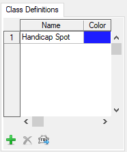
- In the Name field, type Handicap Spot, then click the
 button. The feature is added to the Class Definitions list.
- Click in the color box next to Handicap Spot, and change it to a blue color.
Next, you will select the rasters that you want to train.
Add Training Rasters
- Click the Add button
 below the Rasters section of the Deep Learning Labeling Tool. The Data Selection dialog appears.
- Click the Open File button
 at the bottom of the Data Selection dialog.
- Go to the directory where you saved the tutorial data. Use the Ctrl key to select the following files, then click Open.
- DRCOG_AerialImage1.dat
- DRCOG_AerialImage2.dat
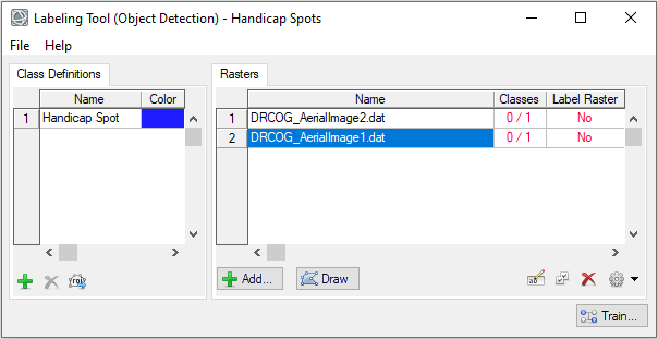
- In the Data Selection dialog, click the Select All button, then click OK.
The training rasters are added to the Rasters section of the Deep Learning Labeling Tool. The table in this section has two additional columns: "Classes" and "Label Raster." Each "Classes" table cell shows a red-colored fraction: 0/1. The "0" means that none of the class labels have been drawn yet. The "1" represents the total number of classes defined. The "Label Raster" column shows a red-colored "No" indicating that no label rasters have been created yet.
For this tutorial, you will restore annotations that were already drawn for each training raster, then add a few more annotations to one of the rasters.
Restore Annotations
- In the Labeling Tool, select DRCOG_AerialImage1.dat.
- Click the Options button
 and select Import Annotations. The Select Annotation Filename dialog appears.
- From the directory that contains the saved tutorial data, select Handicap_Parking_Spots1.anz and click Open. The Match Input Annotations to Class Definitions dialog appears.
- Click the Handicap Spot button. A red line is drawn between AnnotationRectangle and Handicap Spot.
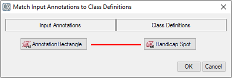
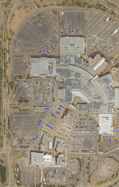
- Click OK. After several seconds, the annotations and image appear in the display. The rectangle annotations are in blue. They surround handicap symbols painted on the pavement throughout the image:
- In the Labeling Tool, select DRCOG_AerialImage2.dat.
- Click the Options button and select Import Annotations.
- Select Handicap_Parking_Spots2.anz and click Open.
- In the Match Input Annotations to Class Definitions dialog, click the Handicap Spot button. A red line is drawn between AnnotationRectangle and Handicap Spot.
- Click OK. After several seconds, the last image and annotations are removed from the display, while the new image and annotations are displayed:
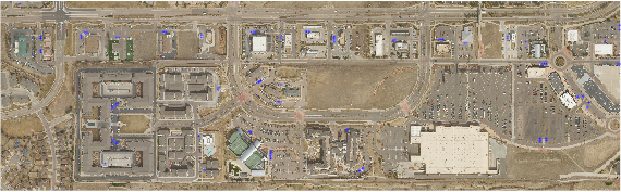
The Labeling Tool now reports 1 out of 1 classes defined for each image. The Layer Manager lists the most recent image that you opened in the Labeling Tool (DRCOG_AerialImage2.dat) and the most recent annotation file you restored. This layer is named "Object Detection Labels."
- Zoom into the image and explore the annotations and objects. You can see how the blue bounding boxes surround the handicap markings.
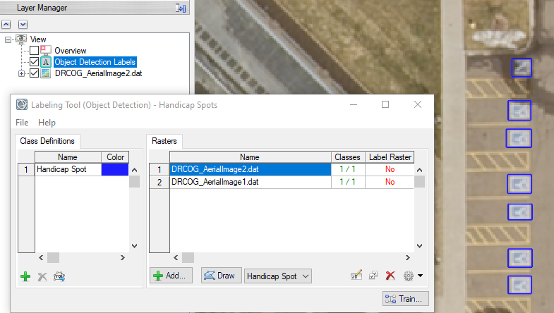
- Double-click Object Detection Labels in the Layer Manager. The Metadata Viewer appears. It shows that this annotation layer contains 84 records, or bounding boxes.
- Close the Metadata Viewer.
Next, you will manually label a few more handicap spots that were missed in the first image.
Label More Objects
-
In the Labeling Tool, select DRCOG_AerialImage1.dat.
-
Click the Draw button. The first image and annotations are displayed.
-
In the Layer Manager, select DRCOG_AerialImage1.dat to make it the active layer.
-
From the Stretch Type drop-down list in the ENVI toolbar, select Optimized Linear. This applies a linear stretch to the image. It provides more contrast to features.
-
Click the Zoom drop-down list in the ENVI toolbar and select 400% (4:1).
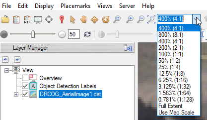
-
In the Go To field in the ENVI toolbar, enter these pixel coordinates: 28981p, 73399p. Be sure to include the "p" after each value. Then press the Enter key on your keyboard. The display centers over an area with four handicap parking spots:
In the Labeling Tool, a drop-down list lets you select the class for which you will draw annotations. In this case, the list shows the only class available, which is Handicap Spot:
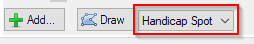
The cursor has also changed to a crosshair symbol, and the Annotation drop-down list in the ENVI toolbar is set to Rectangle. You are now ready to draw more bounding boxes.
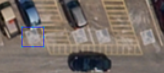
-
Click and hold the left mouse button over the view to draw a box around one of the four handicap signs. Be sure to include all of the painted sign. When you release the mouse button, the box becomes blue. Cyan-colored selection handles around the box let you adjust the box size in any direction.
-
Click and hold the left mouse button to draw boxes around the remaining three handicap signs. To clear the selection handles from the fourth box, click anywhere in the display.
Labeling is now complete, and you can begin the training process.
Train an Object Detection Model
Training involves repeatedly exposing label rasters to a model. Over time, the model will learn to translate the spectral and spatial information in the label rasters into a classification image that maps the features it was shown during training.
- From the Train drop-down list
 at the bottom of the Labeling Tool, select Object Detection. The Train Deep Learning Object Detection Model dialog appears.
-
Keep the Architecture parameter set to RT-DETRV2-Small. This architecture uses a ResNet-18 backbone and performs well when training data is limited.
- The Training/Validation Split (%) slider specifies what percentage of data to use for training versus testing and validation. Keep the default value of 80%.
- Enable the Shuffle Rasters option.
- The remaining parameters provide specialized control over the training process. To learn more about these parameters, click the blue help button in the lower-left corner of the training dialog. For this tutorial, use the following values:
- Number of Epochs: 200
- Patches per Batch: 2
- Background Patch Ratio: 0.15
- Learning Rate: 1e-4
- Gradient Max Normalization: 1.0
- Pad Small Features: Yes
- Augment Scale: Yes
- Augment Rotation: Yes
- Augment Flip: No
- In the Output Model field, choose an output folder and name the model file TrainedModel.envi.onnx, then click Open. This will be the "best" trained model, which is the model from the epoch with the lowest validation loss.
- Leave the Output Last Model field blank.
- Click OK. In the Labeling Tool, the Label Raster column updates with "OK" for all training rasters, indicating that ENVI has automatically created label rasters for training. These label rasters are also called object detection rasters. They look identical to the input rasters, but have additional metadata about the bounding box annotations.
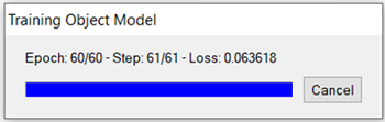
- As training progresses, a Training Model dialog reports the current Epoch, Step, and Loss. You can track how complete each epoch is by watching the steps. For this example, when step is 61/61, the epoch will increase once all steps for the current epoch have completed:
Also, a TensorBoard page displays in a new web browser. This is described next, in View Training Metrics.
Training a model takes a significant amount of time due to the computations involved. Processing can take several minutes to a half-hour to complete, depending on your system hardware and GPU. If you do not want to wait that long, you can cancel the training step now and use a trained model (ObjectDetectionModel_HandicapSpots.envi.onnx) that was created for you, later in the classification step. This file is included with the tutorial data.
View Training Metrics
TensorBoard is a visualization toolkit. It reports real-time metrics during training. Refer to the TensorBoard online documentation for details on its use.
Follow these steps:
-
Set the Smoothing value on the left side of TensorBoard to 0.999. This will allow you to visualize the lines for batch, train, and validation more clearly. Smoothing is a visual tool to help see the entire training session briefly and provide insight into model convergence. Setting smoothing to 0.0 will provide normal values for the given step of a batch for the given epoch.
-
After the first few epochs are complete, TensorBoard provides data for the training session. Several metrics provide insight to how the model is conforming to the data. Scalar metrics include overall and individual class accuracy, precision, and recall. To start, click on Loss in TensorBoard to expand and view a plot of training and validation loss values. Loss is a unitless number that indicates how closely the classifier fits the validation and training data. A value of 0 represents a perfect fit. The farther the value from 0, the worse the fit. Loss plots are provided per batch and per step. Ideally, the training loss values reported in the train loss plot should decrease rapidly during the first few epochs, then converge toward 0 as the number of epochs increases. The following image shows a sample loss plot during a training session of 60 epochs. Your plot might look different:
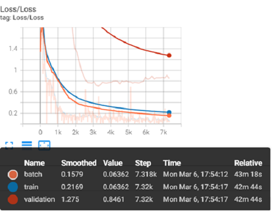
Move the cursor from left to right in the plot to show different values per step.
Batch steps are listed along the X-axis, beginning with 0. A step is calculated with the following equation, (nSteps * nEpochs) * nPatchesPerBatch. For this tutorial nSteps is 61 steps per epoch, epochs are 60, and Patches Per Batch is 2. (60 * 61) * 2 evaluates to 7,320 total training steps. This can be seen in the image above, under Step, 7.32k for train and validation.
-
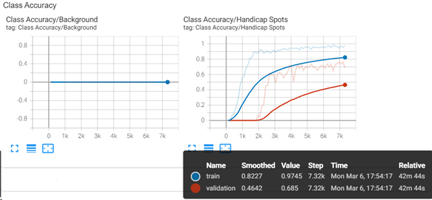
Click Class Accuracy in TensorBoard to view a plot of training and validation accuracy values. The class Background (left plot) is flat along the X axis because ENVI Deep Learning does not retain background patches that are randomly selected from patches without class labels. In the plot on the right, the slope for train and validation starts at 0 and ideally converges toward 1. This is a good indicator that the model is learning the labeled objects. More data, and training for more epochs would improve the results of this output.
-
In the TensorBoard menu bar, click IMAGES.
-
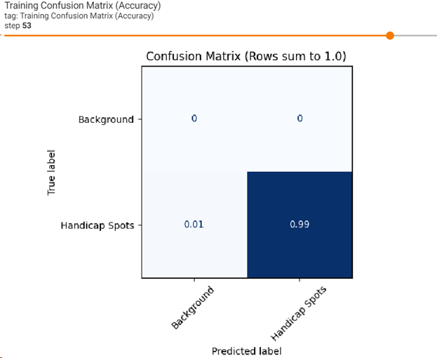
From this option, you can view a confusion matrix for training and validation. Click on the Training Confusion Matrix image to make it larger. Background will display flat at 0 as described previously. By default, the dashboard shows the image summary for the last logged step or epoch. Use the slider to view earlier confusion matrices. In the image below, training is 0.99 percent sure about Handicap Spots for the last epoch, which is a good indicator. Your results might be different:
-
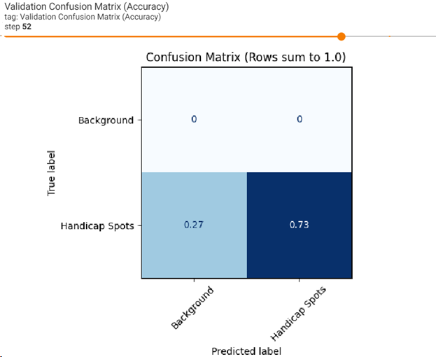
Click on the Validation Confusion Matrix image to make it larger. Validation for Handicap Spots is less confident at 0.73 percent. This is an indicator that the model could benefit by using more data and a longer training session:
-
The full breadth of all metrics is beyond the scope of this tutorial. You can explore the other metrics not covered in this tutorial. See the menu options SCALARS, DISTRIBUTIONS, HISTOGRAMS, and TIME SERIES. When you are finished evaluating training and accuracy metrics:
-
Close the TensorBoard page in your web browser.
-
Close the Labeling Tool. All files and annotations associated with the "Handicap Spot" project are saved to the Project Files directory when you close the tool.
Perform Classification
Now that you have a model that was trained to find examples of handicap parking spots, you will use the same model to find similar instances in a different aerial image of the same region. This is one of the benefits of ENVI Deep Learning; you can train a model once and apply it multiple times to other images that are spatially and spectrally similar. The output will be a shapefile of bounding boxes around features identified as "handicap spot."
-
Select File > Open from the ENVI menu bar.
-
Go to the location where you saved the tutorial data and select the file ImageToClassify.dat. The image appears in the display.
-
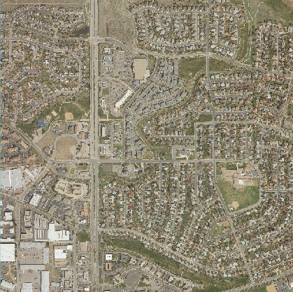
Press the F12 key on your keyboard to zoom out to the full extent of the image. It covers a region that is adjacent to the shopping mall and includes residential neighborhoods. The image was acquired from the same sensor and on the same day.
-
In the Deep Learning Guide Map, click the Back button.
-
Click the Object Classification button. The Deep Learning Object Classification dialog appears. The Input Raster field is already populated with the file ImageToClassify.dat.
-
Click the Browse button next to Input Trained Model. Go to the location where you saved the file TrainedModel.envi.onnx and select that file. (Or, if you skipped training, select the file ObjectDetectionModel_HandicapSpots.envi.onnx included with the tutorial data.) Click Open.
-
Set the Confidence Threshold value to 0.51. By setting this to a median value, the risk of finding false positives (features that are not really handicap spots) is much lower. If you were to set this to a low value, the classifier would find more false positives, resulting in more bounding boxes throughout the scene.
-
Set the Intersection Over Union Threshold value to 0.50. Decrease this value if you experience many overlapping boxes. The model architecture does a good job distinguishing the individual features so it is unlikely that will occur.
-
Select Yes for Enhance Display. This will perform a small linear stretch to the raster before running object classification. Since the input raster is already RGB, you can leave the default value for Visual RGB as No.
-
In the Output Classification Vector field, specify a filename of HandicapSpots.shp.
-
Enable the Display result option.
-
Click OK. When processing is complete, the shapefile appears in the display, overlaid on the image.
-
In the Layer Manager, select HandicapSpots.shp to make it the active layer. The lower-left corner of the ENVI application shows the property sheet for the shapefile.
-
In the property sheet, click the Line Color field, click the drop-down arrow that appears, and select a blue color. The shapefile color changes to blue.
-
Zoom into the image and evaluate the results. Did the classifier find most of the handicap parking spots in the image? Did it identify other features in addition to handicap spots (for example, cars or swimming pools)? If you find that it did not classify enough handicap spots, you could repeat the classification step or click the Postprocess Classification Vector button in the Guide Map. That tool lets you choose different classification values and preview their results before writing a new shapefile. Refer to the Post-process Classification Vectors help topic for details on using that tool.
The following images show examples of the classifier locating handicap parking spots. Your results may be slightly different.

-
When you are finished, exit ENVI.
Final Comments
In this tutorial you learned how to use ENVI Deep Learning to extract one feature from imagery using rectangle annotations to label the features. Once you determine the best parameters to train a deep learning model, you only need to train the model once. Then you can use the trained model to extract the same feature in other, similar images.
In conclusion, deep learning technology provides a robust solution for learning complex spatial and spectral patterns in data, meaning that it can extract features from a complex background, regardless of their shape, color, size, and other attributes.
For more information about the capabilities presented here, refer to the ENVI Deep Learning Help.