Deep Learning Optimized Pixel Classification
Tutorial: Optimized Pixel Classification Using Grid Tutorial
The Deep Learning Optimized Pixel Classification tool uses a trained ENVI Deep Learning pixel segmentation model to perform inference on a raster in regions that contain features of interest identified by a trained ENVI Deep Learning grid model (patent pending). Run this tool as many times as needed to classify multiple rasters. The result is a classification image and a grid output vector.
You can also write a script to classify a raster using the DeepLearningOptimizedPixelClassification task.
Follow these steps:
-
In the ENVI Toolbox, select Deep Learning > Grid > Deep Learning Optimized Pixel Classification. The Deep Learning Optimized Pixel Classification dialog appears with the Main tab selected.
- In the Input Raster field of the Deep Learning Pixel Classification tool, select a raster to classify. It must contain at least as many bands as the raster that was used to train the model.
- In the Input Pixel Model field, select an ONNX file (.envi.onnx) to use for pixel-level classification in the grid-detected cells.
- In the Input Grid Model field, select an ONNX file (.envi.onnx) that was designed for grid-based analysis to classify the input raster.
- For the Confidence Threshold, use the slider bar or up/down arrow buttons to specify a threshold value between 0 and 1.0. Bounding boxes with a confidence score less than this value will be discarded. The default value is 0.2. Decreasing this value generally results in more classification bounding boxes throughout the scene. Increasing it results in fewer classification bounding boxes.
-
For Enhance Display, select Yes if you want to apply an additional small stretch to the processed data to suppress noise and enhance feature visibility. The optional stretch is effective for improving visual clarity in imagery acquired from aerial platforms or sensors with higher noise profiles.
-
For Visual RGB, select Yes if you want to encode the output raster as a three-band RGB composite (red, green, blue) for color image processing. This ensures consistent band selection from ENVI display types (such as RGB, CIR, and pan) and supports integration of diverse data sources (such as MSI, panchromatic, and VNIR) without band mismatch.
- In the Output Classification Raster field, select a path and filename for the output classification raster (.dat). You must specify this or the Output Class Activation Raster, or both.
-
Enable the Display result check box to display the output in the view when processing is complete.
- In the Output Class Activation Raster field, select a path and filename for the output class activation raster (.dat). This is a grayscale image, one band per feature, that shows the probability of pixels belonging to the features of interest.
- Enable the Display result check box to display the output in the view when processing is complete.
- In the Output Classification Vector field, select a path and filename for the output shapefile (.shp). The shapefile contains bounding boxes for each class.
- To set advanced parameters for processing, select the Advanced tab.
-
In the Exclude Classes field, specify the class labels to exclude from the output classification results. This will filter out the specified labels to provide a more targeted and customized output.
-
From the Processing Runtime field, select one of the following execution environments for the classification task:
- CUDA: (Default) Uses NVIDIA GPU acceleration for optimal performance and faster processing
- CPU: Ensures compatibility on systems without GPU support, but with reduced processing speeds.
-
Use the CUDA Device ID parameter to explicitly control GPU selection in multi-GPU environments when you choose CUDA as the Processing Runtime. Optionally enter a target GPU device ID. If you provide a valid ID, the classification task will execute on the specified CUDA-enabled GPU. If the ID is omitted or invalid, the system defaults to GPU device 0.
- Enable the Display result check box to display the output in the view when processing is complete.
-
To reuse these task settings in future ENVI sessions, save them to a file. Click the down arrow  next to the OK button and select Save Parameter Values, then specify the location and filename to save to. Note that some parameter types, such as rasters, vectors, and ROIs, will not be saved with the file. To apply the saved task settings, click the down arrow and select Restore Parameter Values, then select the file where you previously stored your settings.
-
To run the process in the background, click the down arrow and select Run Task in the Background. If an ENVI Server has been set up on the network, the Run Task on remote ENVI Server name is also available. The ENVI Server Job Console will show the progress of the job and will provide a link to display the result when processing is complete. See the ENVI Servers topic in ENVI Help for more information.
- Click OK. ENVI adds the resulting output to the Data Manager and Layer Manager.
Evaluate the Results
Optimized pixel segmentation is the process of first eliminating unnecessary portions of the raster quickly. Using grid, you can determine the areas of the raster that contain zero features of interest. Once valid areas of interest are outlined by grid, you can apply pixel classification to those areas.
The example image below was generated with the Grid_Tutorial_Data content that can be downloaded from our ENVI Tutorials web page. The grid tutorial data provides a NAIP dataset with boats that have been labeled with points using ENVI’s Labeling Tool. The input classification raster is \Classification\Rasters\massachusetts_1_20100821.tif
The following input models are in Grid_Tutorial_Data\Classification\Models:
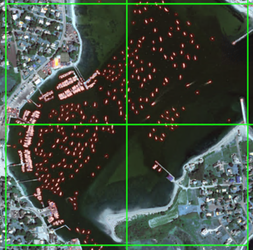
The output image below was generated by enabling the Display result check boxes under the Output Classification Raster and Output Classification Vector. The Confidence Threshold was set to 0.90, to detect only features with a 90% accuracy rating.
Follow these steps to overlay the output classification raster and vector over the Input Raster:
- Display the Input Raster in the current view.
- In the Layer Manager, click and drag the Input Raster below the raster and vector classification outputs.
-
To view the input raster, clear the check box for the 0: Unclassified class of the output classification raster in the Layer Manager.
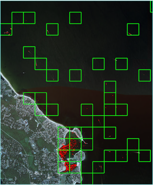
The view should now be identical to the image above. When zoomed out to the extents of the input raster, you will see green boxes representing grid detections, and red pixels representing pixel classification.
-
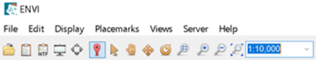
Zoom in to the image for a closeup of the results. In the Layer Manager, select the output vector classification and change the zoom to 1:10,000 from the Zoom drop-down list, highlighted in blue in the image below.
-
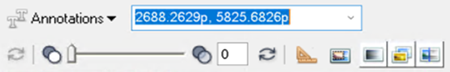
In the Go To field, enter the following coordinates and press the Enter key: 2688.2629p, 5825.6826p, highlighted in the next image.
-
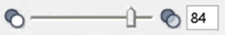
To see the classified features that are under the red pixel segments, select the output classification raster in Layer Manager, then move the Transparency slider back and forth to see the underlying feature. A transparency value of 84 is good for viewing features while still easily seeing the red classification pixels.
The example above displays multiple boats docked and in open water. Zoom in for a closer look.
- Use the output vector classification to determine the confidence of features detected in a given grid cell. This will help determine how well the model did and help guide additional classification using a higher or lower confidence threshold. In the Layer Manager, select the output classification vector, then right-click, and select Filter Records by Attributes.
-
In the Filter by Attributes dialog, select the Class_ID drop-down list, then select Confidence.
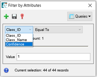
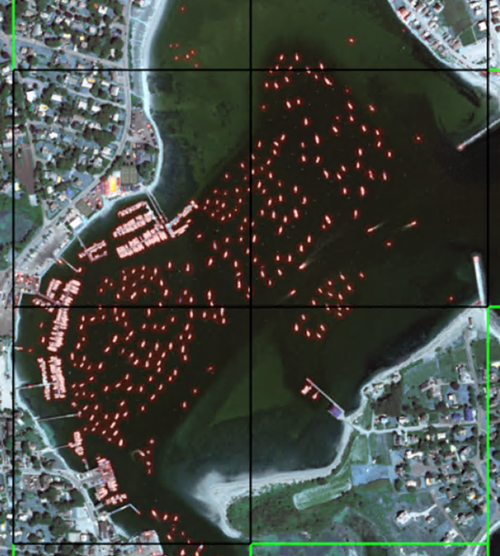
- Move the slider bar to the far right to set the confidence Value to 0.999. Green squares will turn black to show the areas with the selected confidence value.
-
If the view is still centered on the coordinates, you will see three grid cells highlighted in black and a partial top-right grid cell in black shown in the image. All black grids are 0.999 confidence of the features within in them.
See Also
Train Deep Learning Pixel Models, Train Deep Learning Grid Models, Deep Learning Grid Classification