Dynamic PLOT Visualizations

The PLOT function's Equation argument (and the EQUATION property) adds a level of flexibility to the creation of plots. This topic explores ways you can use the Equation argument to create dynamic, interactive plots.

The Equation argument on the PLOT function allows you to specify either a string containing an equation with variable X, or the name of an IDL function that accepts X as an input argument. The result of the equation (or the function) should be a one-dimensional array of Y coordinates to be plotted.

If Equation is an expression, then the EXECUTE function is called once with the X array. Note that in certain circumstances (such as the IDL Virtual Machine), you may not be able to use the EXECUTE function.
If Equation is a function name, then CALL_FUNCTION is called once, with the X array as an input argument. The function should return a one-dimensional result array.

Once IDL creates the plot output, if you then interactively adjust the plot range, IDL will automatically recompute the equation to cover the new range.

Using an Equation String

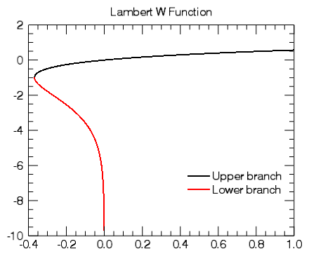
For the first example, we will have IDL plot the LAMBERTW function:

p1 = PLOT('LambertW(x)', '2', DIMENSIONS=[400,400],$

  NAME='Upper branch', $

  TITLE='Lambert W Function', XRANGE=[-0.4, 1])

p2 = PLOT('LambertW(x, /LOWER_BRANCH)', '2r', /OVERPLOT, $

  NAME='Lower branch')

lg = LEGEND(/DATA, POSITION=[0.95, -6], LINESTYLE=6, SHADOW=0)

This should produce the following graphic:

Once IDL creates the plot, test out its dynamic capabilities:

Try clicking with the middle mouse button on the graphic and panning around.
You can also use the mouse wheel to zoom in or out, or hold down the <Shift> key and draw a zoom box.
Try programmatically changing the plot range at the IDL command line:

  p1.XRANGE = [-0.5, 0.5]

  p1.YRANGE = [-2, 1]

In all of these cases, as you change the plot range, IDL recomputes the equation with new X values that span the new range.

Using an Equation Function

Using an equation string has some limitations:

You can only have a single statement.
You cannot easily change the equation unless you set a new string.
You cannot pass parameters into your equation.

As a different approach, create an IDL function containing your equation and then pass the function name to the Equation argument. This method allows you a bit more flexibility in your input equations.

For example, in the first line of the code above, we could have written:

p1 = PLOT('LambertW', '2', DIMENSIONS=[400,400],$

  NAME='Upper branch', $

  TITLE='Lambert W Function', XRANGE=[-0.4, 2])

Notice that we no longer have an X variable in our equation, we just have the name of the function.

We can also create our own routine which accepts our X vector and some optional user data.

First, create a new IDL routine called ex_plot_function and save it in a file ex_plot_function.pro on IDL's path:

FUNCTION ex_plot_function, x, k

  COMPILE_OPT IDL2

  RETURN, LAMBERTW(DCOMPLEX(x), k)

END

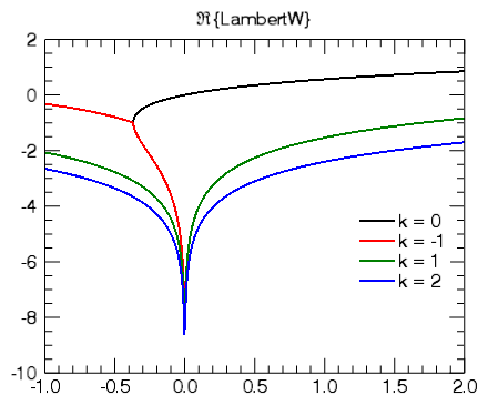
Next, we create our plot visualization, passing in the name of our equation along with our user data containing the "branch" parameter k:

p1 = PLOT('ex_plot_function', '2', DIMENSIONS=[400,400],$

  NAME='k = 0', EQN_USERDATA=0, $

  TITLE='$\Re${LambertW}', XRANGE=[-1, 2])

p2r = PLOT('ex_plot_function', '2r', /OVERPLOT, $

  NAME='k = -1', EQN_USERDATA=-1)

p3r = PLOT('ex_plot_function', '2g', /OVERPLOT, $

  NAME='k = 1', EQN_USERDATA=1)

p4r = PLOT('ex_plot_function', '2b', /OVERPLOT, $

  NAME='k = 2', EQN_USERDATA=2)

lg = LEGEND(/DATA, POSITION=[1.9, -4], LINESTYLE=6, SHADOW=0)

Our plot should now look like the following:

Again, we can pan and zoom around the plot, and IDL will automatically update the equations.

Product	IDL

Version	9.0