If you create an Image graphic by projecting a graphic file onto a map, you can convert the IDL graphic into other graphic types, including the Open Geospatial Consortium's Keyhole Markup Language (KML). KML is an XML-based schema that visualizes geographic data and annotations on Internet-based two-dimensional maps and three-dimensional Earth browsers (including the Google Earth™ mapping service).
This topic shows how to use a graphic's Save method to convert an Image graphic to a KML file.
Arctic Research Flight Example
In this example we project a portion of a JPG image of the world onto a globe, and add a line showing a research airplane's flight path between Thule Air Force Base in Greenland and Alaska's Elmendorf Air Force Base. We also add a polygon to the Image graphic showing the magnetic anomaly detected during the flight. Finally, we save this Image graphic with the added annotations to a KML file and load the file into the Google Earth™ mapping service.
This code creates a KML file that, when loaded into the Google Earth™ mapping service, creates the image shown above. You can copy the entire block and paste it into the IDL command line to run it.
world = FILEPATH('Day.jpg', SUBDIRECTORY=['examples','data'])
arctic = IMAGE(world, LIMIT=[51,-161,78,-52], $
GRID_UNITS=2, IMAGE_LOCATION=[-180,-90], $
IMAGE_DIMENSIONS=[360,180], MAP_PROJECTION='Stereographic', $
/CURRENT, NAME='Arctic Research')
polyline = POLYLINE([[-149.81,61.25],[-68.70,76.53]], $
/DATA, COLOR='red', NAME='Thule to Elmendorf', $
THICK=2, TARGET=arctic)
x = [-119.017, -124.82, -129.22, -118.23, -113.03, -113.183]
y = [66.25, 64.65, 61.43, 62.3, 63.783, 65.11]
polygon = POLYGON(x, y, /DATA, COLOR='purple', $
FILL_COLOR='purple', FILL_TRANSPARENCY=0, $
NAME='Magnetic Anomaly', TARGET=arctic)
arctic.SAVE, 'arctic_map.kml'
In this example we start with the two-dimensional Day.jpg file (included in the IDL distribution):
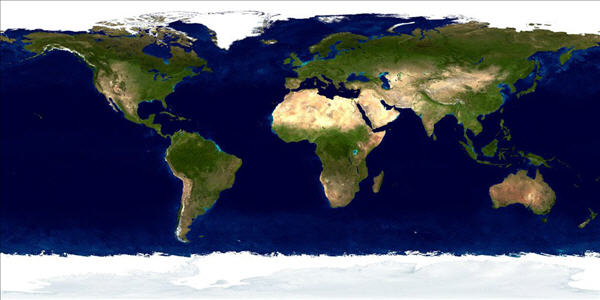
world = FILEPATH('Day.jpg', SUBDIRECTORY=['examples','data'])
We then call the IMAGE function,which does the following things:
- Maps the two-dimensional Day.jpg using a stereographic projection
- Defines a polygon on the globe using the two opposing corner coordinates
- Maps the polygon back to a two-dimensional surface
arctic = IMAGE(world, LIMIT=[51,-161,78,-52], $
GRID_UNITS=2, IMAGE_LOCATION=[-180,-90], $
IMAGE_DIMENSIONS=[360,180], MAP_PROJECTION='Stereographic', $
/CURRENT, NAME='Arctic Research')
Next we add a polyline annotation representing the research airplane's flight path, and a polygon showing the magnetic anomaly detected on the flight:
polyline = POLYLINE([[-149.81,61.25],[-68.70,76.53]], $
/DATA, COLOR='red', NAME='Thule to Elmendorf', $
THICK=2, TARGET=arctic)
x = [-119.017, -124.82, -129.22, -118.23, -113.03, -113.183]
y = [66.25, 64.65, 61.43, 62.3, 63.783, 65.11]
polygon = POLYGON(x, y, /DATA, COLOR='purple', $
FILL_COLOR='purple', FILL_TRANSPARENCY=0, $
NAME='Magnetic Anomaly', TARGET=arctic)
The resulting Image graphic shows the polygon section of the globe projected stereographically:
Finally, we save the Image graphic as a KML file using the Image object's Save method and load the file into the Google Earth™ mapping service, where it is superimposed upon a globe.
ContourExample
In this example we create a map of the world using the Mollweide projection, and overplot that map with two 3-D contour plots (one that displays filled contour levels with different colors, and one that just shows the contour boundaries). We then use the CONTOUR function's SAVE method to create a KML file and load the file into the Google Earth™ mapping service.
This code creates a KML file that creates the image shown above. You can copy the entire block and paste it into the IDL command line to run it.
longitude = FINDGEN(360) - 180
latitude = FINDGEN(180) - 90
cntrdata = SIN(longitude/30) # COS(latitude/30)
worldmap = MAP('Mollweide', LIMIT=[-90,-180,90,180])
cntr1 = CONTOUR(cntrdata, longitude, latitude, $
GRID_UNITS=2, N_LEVELS=10, RGB_TABLE=13, /OVERPLOT, $
/FILL, TRANSPARENCY=50)
cntr2 = CONTOUR(cntrdata, longitude, latitude, $
GRID_UNITS=2, N_LEVELS=10, RGB_TABLE=39, $
/OVERPLOT, C_THICK=[2])
worldmap.SAVE, 'contour_map.kml'
At this point you can load contour_map.kml into the Google Earth™ mapping service, and the map and overplotted contour plots are projected on a globe.
Resources