You can add or change axes in graphics. The examples on this page include adding axes to an image and adding and changing the properties of an axis on a three-dimensional contour graphic.
Add Axes to an Image
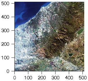
Axes on an image help illustrate the dimensions (number of pixels) in each direction, as shown in the following example:
aerial_view = FILEPATH('elev_t.jpg', $
SUBDIR=['examples','data'])
im = IMAGE(aerial_view, DIMENSIONS=[400, 400], MARGIN=0.2)
xax = AXIS('X', LOCATION='bottom', TICKDIR=1, MINOR=0)
yax = AXIS('Y', LOCATION='left', TICKDIR=1, MINOR=0)
Add Axes to a 3D Contour
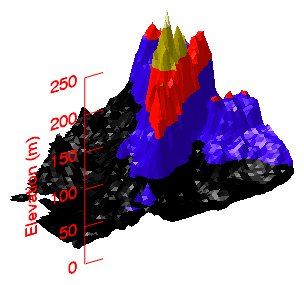
The example shows a digital elevation model (DEM) taken from the Santa Monica mountains in California. This three-dimensional example illustrates how to add a Z axis to the graphic after creation.
file = file_which('elevbin.dat')
dem = read_binary(file, data_dims=[64, 64])
c = CONTOUR(dem, $
RGB_TABLE=5, $
/FILL, $
PLANAR=0, $
AXIS_STYLE=0)
z = AXIS('Z', LOCATION=['left', 'bottom'])
z.MINOR = 0
z.TICKLEN = 0.10
z.COLOR = 'red'
z.TITLE = 'Elevation (m)'
Add Custom Axes with a User-defined Range
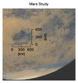
Axes may also be added at arbitrary locations, and with custom offset and scale factors. For example:
file = FILEPATH('marsglobe.jpg', $
SUBDIRECTORY = ['examples', 'data'])
mglobe = IMAGE(file, TITLE='Mars Study', $
XRANGE=[175, 325], YRANGE=[0, 150], $
TRANSPARENCY=20)
marsDiameter = 6792
scaleFactor = marsDiameter/400
ax1 = AXIS('x', LOCATION=70, $
TITLE='(km)', $
/DATA, $
AXIS_RANGE=[0, 600], $
COORD_TRANSFORM=[-195, 1] * scaleFactor, $
MINOR=0, MAJOR=3)
ax2 = AXIS('y', LOCATION=235, $
TITLE='(km)', TEXTPOS=1, $
/DATA, $
AXIS_RANGE=[0, 500], $
COORD_TRANSFORM=[-75, 1] * scaleFactor, $
MINOR=0, MAJOR=3)
x = findgen(100)/5
y = beselj(x)
myPlot = PLOT(x, y, COLOR='red', NAME='bessel_j0')
Modifying Axes and Their Properties
You can use axis references or the dot notation to change the properties of an axis after the creation of any graphic. For more information on available axis properties, see AXIS(). For general information on graphics properties, see Change Graphics Properties.
Using the Dot Notation
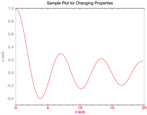
Generate a basic plot and to learn how you can use the dot syntax to change axis properties.
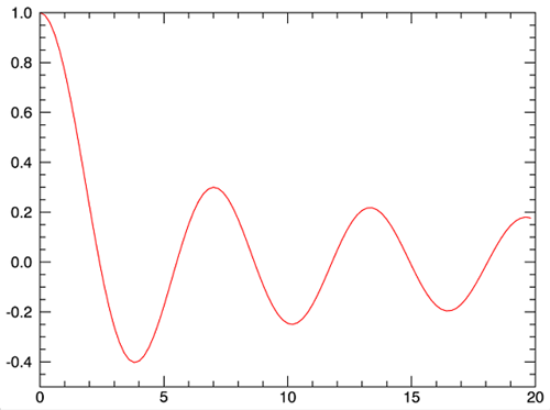
Copy and paste the following code at the IDL command line to generate the plot shown above:
x = findgen(100)/5
y = beselj(x)
myPlot = PLOT(x, y, COLOR='red', NAME='bessel_j0')
To see an explanation of the properties for this plots, see the PLOT function topic. The general syntax for changing graphics properties after creation is:
<graphic_var_name>.PROPERTYNAME = value
You can change the properties of the plot, using the variable name of the plot along with the "dot" syntax. The plot graphics here show several of the properties that you can change interactively. Try these commands at the command line to see the changes to the plots:
myPlot.TITLE = "Sample Plot for Changing Properties"
myPlot.XTITLE= "x-axis
myPlot.YTITLE = "y-axis"
myPlot.XTICKLEN = .02
myPlot.YTICKLEN = .02
myPlot.XTEXT_COLOR = 'red'
myPlot.YTRANSPARENCY = 50
myPlot.YTRANSPARENCY = 25
myPlot.YTRANSPARENCY = 75
myPlot.XTRANSPARENCY = 0
Your graphic should now look like this:
Using Axis References and Hash Notation
You can also use axis references and the hash notation to change the properties of specific axes. Remember that in a two-dimensional plot, the primary x-axis is numbered zero ("0") and the remaining axes are numbered clockwise, incrementally.
myPlot['axis0'].TITLE = 'X-axis'
myPlot['axis1'].TITLE = 'Y-axis'
myPlot['axis1'].COLOR = 'forest green'
myPlot['axis1'].TRANSPARENCY = 0
myPlot['axis3'].TITLE = 'Second y-axis'
myPlot['axis3'].SHOWTEXT = 1
myPlot['axis3'].TRANSPARENCY = 80
myPlot['axis3'].TRANSPARENCY = 90
myPlot['axis2'].TRANSPARENCY = 90
One advantage of using the hash notation with numeric axis references is that you can easily change the properties of the secondary x- and y-axes. This notation also works with three-dimensional graphics. See Axis References in IDL Graphics for more information.
See Also