The SURFACE function's Equation argument (and the EQUATION property) adds flexibility to the creation of surface plots. This topic explores ways you can use the EQUATION property to create dynamic, interactive surface visualizations.

The Equation argument on the SURFACE function allows you to specify either a string giving an equation of X and Y, or the name of an IDL function that accepts X and Y as arguments. The result of the equation (or the function) should be a two-dimensional array of Z coordinates giving the surface heights.

• If Equation is an expression, then IDL calls the EXECUTE function once with the X and Y arrays. Note that in certain circumstances (such as the IDL Virtual Machine), you may not be able to use the EXECUTE function.
• If Equation is a function name, then CALL_FUNCTION is called once, with the X and Y arrays as input arguments. The function should return a two-dimensional result array.

Once IDL creates the surface visualization, if you then programmatically adjust the surface X and Y ranges, IDL will automatically recompute the equation to cover the new range.

Since the Equation functionality on SURFACE is so similar to the CONTOUR function, we will skip the simple example in favor of a more complicated example using an IDL function.

Using an Equation Function

---

First, create a new IDL routine called ex_surface_function and save it in a file ex_surface_function.pro on IDL's path:

function ex_surface_function, x, y, userdata

  z = x + !const.I*y

  k = userdata.k

  result = LambertW(z, k)

  result = userdata.real ? Real_Part(result) : Imaginary(result)

  result[WHERE(ABS(z) gt 5, /NULL)] = !values.d_nan

  return, result

end

Note that we are passing in the "branch" parameter k and the real/imaginary flag in USERDATA, so that we can easily modify these parameters later.

Next, create our surface visualization by passing in the name of our equation and our specific userdata for each surface call:

s1 = SURFACE('ex_surface_function', STYLE=0, LAYOUT=[2,1,1], $

  EQN_USERDATA={real:1, k:0}, EQN_SAMPLES=100, ZRANGE=[-4,2], $

  ASPECT_RATIO=1)

s2 = SURFACE('ex_surface_function', STYLE=0, /OVERPLOT, $

  EQN_USERDATA={real:1, k:1}, EQN_SAMPLES=100, COLOR='blue')

s3 = SURFACE('ex_surface_function', STYLE=0, /OVERPLOT, $

  EQN_USERDATA={real:1, k:2}, EQN_SAMPLES=100, COLOR='green')

s4 = SURFACE('ex_surface_function', STYLE=0, /OVERPLOT, $

  EQN_USERDATA={real:1, k:3}, EQN_SAMPLES=100, COLOR='red')

s5 = SURFACE('ex_surface_function', STYLE=0, LAYOUT=[2,1,2], $

  EQN_USERDATA={real:0, k:0}, EQN_SAMPLES=100, /CURRENT, $

  ASPECT_RATIO=1)

s6 = SURFACE('ex_surface_function', STYLE=0, /OVERPLOT, $

  EQN_USERDATA={real:0, k:1}, EQN_SAMPLES=100, COLOR='blue')

s7 = SURFACE('ex_surface_function', STYLE=0, /OVERPLOT, $

  EQN_USERDATA={real:0, k:2}, EQN_SAMPLES=100, COLOR='green')

s8 = SURFACE('ex_surface_function', STYLE=0, /OVERPLOT, $

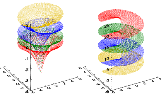
  EQN_USERDATA={real:0, k:3}, EQN_SAMPLES=100, COLOR='red')

This produces the following graphic:

Other Topics in this Series

---

• Dynamic Plot Visualizations
• Dynamic Contour Visualizations

See Also

---

COLORBAR, SURFACE, WINDOW, Graphics Event Handlers