In this topic we explore how to combine two different SURFACE plots with POLYLINE and SCATTERPLOT3D to further characterize the study area. We use the same data as in the topic "Model the Study Area and Setting," but view the data as three-dimensional surfaces rather than a two-dimensional contour plot.
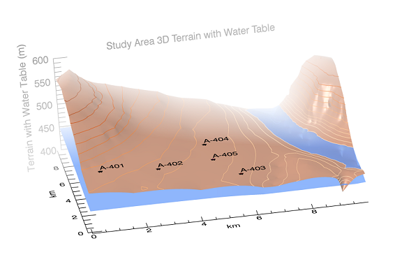
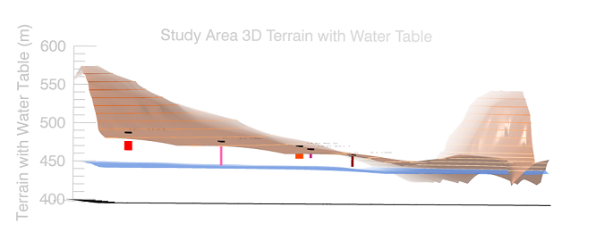
Your resulting graphic should look similar to these depending on how you rotate and resize the plot and window (these plots were stretched in the X dimension):
Read In and Grid the Terrain Data
Start by reading in the base data to use throughout the rest of the examples. The data resides in the file TankDataTerrain.csv in the \examples\data directory of your IDL installation. This file contains the surface terrain data of our site, in X, Y, Z coordinates (all in meters). The fourth column of data in this file contains the elevation of the surface of the underlying aquifer.
In this example, we create a template with ASCII_TEMPLATE, then read in the data using READ_ASCII.
myTemplate = ASCII_TEMPLATE()
site = READ_ASCII('TankDataTerrain.csv', $
TEMPLATE=myTemplate)
grid = GRIDDATA(site.X, site.Y, site.Z, $
DIMENSION=1000, METHOD="Kriging")
Create the Surface Plot
Next, begin creating the surface plot from the gridded terrain data.
The DEPTH_CUE property creates the haze effect in the graphic, above. We use Gouraud shading in this example, and set ASPECT_Z to 2.5 in order to exaggerate the Z-dimension and make the plot easier to view.
mySurf = SURFACE(grid, RGB_TABLE=16, TRANSPARENCY=40, $
COLOR='sienna', DEPTH_CUE=[0,1], SHADING=1, $
TITLE="Study Area 3D Terrain with Water Table", $
ASPECT_RATIO=.75, ASPECT_Z=2.5)
mySurf.TITLE.UPDIR = [0,0,1]
mySurf['axis0'].TRANSPARENCY = 100
mySurf['axis1'].TRANSPARENCY = 100
mySurf['axis2'].TRANSPARENCY = 100
surfXAxis = AXIS('X', LOCATION=-15, TITLE='km', TICKINTERVAL=2, $
COORD_TRANSFORM=[0,0.01])
surfYAxis = AXIS('Y', LOCATION=-15, TITLE='km', TICKINTERVAL=2, $
COORD_TRANSFORM=[0,0.01])
zAxis = AXIS('Z', LOCATION=[0, 1010], TICKINTERVAL=50, $
TITLE='Terrain with Water Table (m)', AXIS_RANGE=[0.0,600])
contours = CONTOUR(grid, C_VALUE=site.Z, PLANAR=0, FONT_SIZE=12, $
C_LABEL_SHOW=0, /OVERPLOT)
gridH2O = GRIDDATA(site.X, site.Y, site.AQ, DIMENSION=1000, $
METHOD="Kriging")
myWaterTable = SURFACE(gridH2O, TRANSPARENCY=25, $
COLOR='cornflower', /OVERPLOT)
Add the Tank and Well Locations to the Plot
Waste was pumped into both wells and storage tanks, so plot these in 3D space in relation to the surface of the water table. We will also plot the locations of the tanks and wells on the actual SURFACE plot.
tank1 = POLYLINE([66,66], [210,210], [475,473], /DATA, $
TARGET=mySurf, COLOR='red', THICK=10)
well2 = POLYLINE([276,276], [221,221], [479,450], /DATA, $
TARGET=mySurf, COLOR='hot pink', THICK=3)
well3 = POLYLINE([566,566], [146,146], [463,450], /DATA, $
TARGET=mySurf, COLOR='dark red', THICK=3)
tank4 = POLYLINE([471,471], [483,483], [465,462], /DATA, $
TARGET=mySurf, COLOR='orange red', THICK=10)
well5 = POLYLINE([484,484], [313,313], [470,460], /DATA, $
TARGET=mySurf, COLOR='medium violet red', THICK=3)
xLoc = [66,276,566,471,484]
yLoc = [210,221,146,483,313]
zLoc = [491,480,463,473,470]
zLocLabels = [495,484,467,477,474]
labels = ['A-401','A-402','A-403','A-404','A-405']
myPlot2 = SCATTERPLOT3D(xLoc, yLoc, zLoc, /OVERPLOT, SYMBOL='*', $
SYM_SIZE=1, SYM_FILLED=1, SYM_THICK=2, SYM_FILL_COLOR='black')
myLabels = TEXT(xLoc, yLoc, zLocLabels, labels, /DATA, /OVERPLOT)
Other Topics in this Series
See Also
ASCII_TEMPLATE, AXIS, CONTOUR, GRIDDATA, POLYLINE, READ_ASCII, READ_CSV, SCATTERPLOT, SCATTERPLOT3D, SURFACE, TEXT