Dynamic Contour Visualizations

The CONTOUR function's Equation argument (and the EQUATION property) adds flexibility to the creation of contour plots. This topic explores ways you can use the EQUATION property to create dynamic, interactive contour visualizations.

The Equation argument on the CONTOUR function allows you to specify either a string giving an equation of X and Y, or the name of an IDL function that accepts X and Y as arguments. The result of the equation (or the function) should be a two-dimensional array of Z coordinates to be contoured.

If Equation is an expression, then IDL calls the EXECUTE function once with the X and Y arrays. Note that in certain circumstances (such as the IDL Virtual Machine), you may not be able to use the EXECUTE function.
If Equation is a function name, then CALL_FUNCTION is called once, with the X and Y arrays as input arguments. The function should return a two-dimensional result array.

Once IDL creates the contour visualization, if you then interactively adjust the contour plot range, IDL will automatically recompute the equation to cover the new range.

Using an Equation String

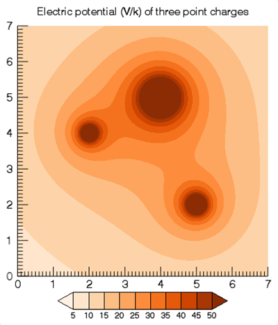
For the first example, we will have IDL compute the electric potential for three point charges. The electric potential of a point charge is given by Gauss's law, V = kQ/r, where Q is the electric charge, k= 8.987x10⁹ V m C^-1 is Coulomb's constant, and r is the distance from the charge.

Here, we will consider three point charges, the first, of 9 coulombs, at location (2, 4), the second, of 12 coulombs at (5, 2), and the third, of 25 coulombs, at (4, 5). To avoid huge values, the value of the electric potential is divided by k.

; Construct our equation as a function of X and Y.

equation = '9/sqrt((x-2)^2 + (y-4)^2) + 12/sqrt((x-5)^2 + (y-2)^2)' + $

  ' + 25/sqrt((x-4)^2 + (y-5)^2)'

; Make the graph with filled contours.

title = 'Electric potential (V/k) of three point charges'

cplot = CONTOUR(equation, XRANGE=[0,7], YRANGE=[0,7], $

  RGB_TABLE=55, /FILL, $

  C_VALUE=[0:50:5], $

  TITLE=title, DIMENSIONS=[800, 800], ASPECT_RATIO=1)

cb = COLORBAR(TARGET=cplot, /BORDER)

This should produce the following graphic:

Once IDL creates the visualization, test out its dynamic capabilities:

Try clicking with the middle mouse button on the graphic and panning around.
Use the mouse wheel to zoom in or out, or hold down the <Shift> key and draw a zoom box.
You can also programmatically change the plot range:

  cplot.XRANGE = [-10, 10]

  cplot.YRANGE = [-10, 10]

In all of these cases, as the contour plot range changes, IDL recomputes the equation with new X and Y values that span the range.

Using an Equation Function

Using an equation string has some limitations:

You can only have a single statement.
You cannot easily change the equation unless you set a new string.
You cannot pass parameters into your equation.

As a different approach, create an IDL function containing your equation and then pass the function name to the Equation argument. We can now repeat the above example using a function.

First, create a new IDL routine called ex_contour_function and save it in a file ex_contour_function.pro on IDL's path:

; This code displays the electric field,

; in terms of voltage, made from three point charges.

FUNCTION ex_contour_function, x, y, userdata

  COMPILE_OPT IDL2

  charge = USERDATA.charge

  xcoord = USERDATA.xcoord

  ycoord = USERDATA.ycoord

  ; Use Gauss's law to convert to an electric potential.

  ; Use >1d-4 to avoid a divide-by-zero at each charge's center.

  v1 = charge[0]/(((x-xcoord[0])^2 + (y-ycoord[0])^2) > 1d-4)

  v2 = charge[1]/(((x-xcoord[1])^2 + (y-ycoord[1])^2) > 1d-4)

  v3 = charge[2]/(((x-xcoord[2])^2 + (y-ycoord[2])^2) > 1d-4)

  ; Build the equation for electric field at any given point.

  RETURN, v1 + v2 + v3

END

Note that we are now passing in the charge values and locations in USERDATA, so that we can easily modify these parameters later.

Next, create our contour visualization by first defining our user data and then passing in the name of our equation:

; Experiment by changing the magnitudes and location of the charges.

userdata = {charge: [9, 12, 25], xcoord: [2d, 5, 4], ycoord: [4d, 2, 5]}

title = 'Electric potential (V/k) of three point charges'

cplot = CONTOUR('ex_contour_function', XRANGE=[0,7], YRANGE=[0,7], $

  RGB_TABLE=55, /FILL, C_VALUE=[0:50:5], $

  EQN_USERDATA=userdata, $

  TITLE=title, DIMENSIONS=[800, 800], ASPECT_RATIO=1)

cb = COLORBAR(TARGET=cplot, /BORDER)

This plot should look identical to the one in the previous section.

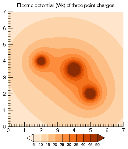
Again, we can pan, zoom, and change the axis range and the contour plot will automatically update to the new ranges. Additionally, we can also change the parameter values and recompute the equation. For example:

USERDATA.charge[2] = 15

USERDATA.ycoord[2] = 3.5

; Reset the user data property to force an update.

cPlot.eqn_userdata = userdata

This produces the following graphic:

Bonus: Interactively Changing the Charges and Locations

The previous two sections demonstrate how to use the Equation argument. This section goes beyond just the Equation argument and explains how to enable mouse and keyboard events to manipulate the point charges.

The code to create the contour remains essentially unchanged from the examples above. For convenience, save the following code within a new file, ex_contour_equation.pro, somewhere on IDL's path:

; Experiment by changing the magnitudes and location of the charges.

userdata = {charge: [9, 12, 25], xcoord: [2d, 5, 4], ycoord: [4d, 2, 5]}

title = 'Electric potential (V/k) of three point charges'

cPlot = CONTOUR('ex_contour_function', XRANGE=[0,7], YRANGE=[0,7], $

  RGB_TABLE=55, /FILL, C_VALUE=[0:50:5], $

  EQN_USERDATA=userdata, $

  TITLE=title, DIMENSIONS=[800, 800], ASPECT_RATIO=1)

cb = COLORBAR(TARGET=cPlot, /BORDER)

oText = TEXT(userdata.xcoord, userdata.ycoord, $

  STRTRIM(userdata.charge, 2), $

  /DATA, ALIGN=0.5, VERTICAL_ALIGN=0.5)

cPlot.WINDOW.EVENT_HANDLER = Ex_Contour_Handler(cPlot, oText)

We are now adding three text objects that display the charge value at each point charge. In addition, we are adding a mouse/keyboard event handler object to the WINDOW's EVENT_HANDLER property.

To create the Ex_Contour_Handler object, save the following code within a file ex_contour_handler__define.pro on IDL's path. Note that there are two underscores in front of the "define" in the filename.

FUNCTION Ex_Contour_Handler::Init, cPlot, oText

  COMPILE_OPT IDL2

  ; Cache our member data.

  self.cPlot = cPlot

  self.oText = oText

  self.hitCharge = -1

  RETURN, 1 ; success

END

FUNCTION Ex_Contour_Handler::MouseDown, oWin, x, y, button, keymods, clicks

  COMPILE_OPT IDL2

  self.hitCharge = -1

  ; User must do a single click with the left button, otherwise return.

  IF (button NE 1 || keymods NE 0 || clicks NE 1) THEN BEGIN

    RETURN, 1  ; default handling

  ENDIF

  ; Did we hit one of our Text graphics? It will always be

  ; the last item in the array since it was added last.

  oVis = (oWin->HitTest(x, y))[-1]

  IF (~ISA(oVis)) THEN RETURN, 1

  self.hitCharge = WHERE(self.oText eq oVis[0])

  self.buttonDown = 1b

  RETURN, 1

END

FUNCTION Ex_Contour_Handler::MouseMotion, oWin, x, y, keymods

  COMPILE_OPT IDL2

  ; Return early if we don't have a charge selected

  IF (self.hitCharge LT 0 || ~KEYWORD_SET(self.buttonDown)) THEN $

    RETURN, 1

  ; Determine the new X/Y coordinates for the charge.

  xy = self.cPlot.ConvertCoord(x, y, /DEVICE, /TO_DATA)

  userdata = self.cPlot.eqn_userdata

  userdata.xcoord[self.hitCharge] = xy[0]

  userdata.ycoord[self.hitCharge] = xy[1]

  ; Reset the user data property to force an update

  self.cPlot.eqn_userdata = userdata

  ; Be sure to move the charge's text string.

  xy = self.cPlot.ConvertCoord(x, y, /DEVICE, /TO_NORMAL)

  self.oText[self.hitCharge].POSITION = xy[0:1]

  RETURN, 1

END

FUNCTION Ex_Contour_Handler::MouseUp, oWin, x, y, button

  COMPILE_OPT IDL2

  IF (self.hitCharge ge 0) THEN BEGIN

  void = self->MouseMotion(oWin, x, y, 0)

  ENDIF

  self.buttonDown = 0b

  RETURN, 1

END

FUNCTION Ex_Contour_Handler::Keyhandler, $

  Window, IsASCII, Character, KeyValue, X, Y, Press, Release, KeyMods

  COMPILE_OPT IDL2

  ; Return early if no charge has been selected

  IF (self.hitCharge LT 0 || ~Press) THEN RETURN, 1

  ch = STRING(character)

  IF (ch eq '=' || ch eq '+' || ch eq '-') THEN BEGIN

    userdata = self.cPlot.eqn_userdata

    ; Press + key to increase charge, - key to decrease

    userdata.charge[self.hitCharge] += (ch eq '-' ? -1 : 1)

    ; Reset the user data property to force an update

    self.cPlot.eqn_userdata = userdata

    ; Be sure to update the charge's text string.

    self.oText[self.hitCharge].STRING = $

    STRTRIM(userdata.charge[self.hitCharge],2)

  ENDIF

  RETURN, 1

END

PRO Ex_Contour_Handler__define

  void = {Ex_Contour_Handler, inherits GraphicsEventAdapter, $

    cPlot: OBJ_NEW(), $

    oText: OBJARR(3), $

    hitCharge: 0, $

    buttonDown: 0b}

END

Now run your main procedure:

.run ex_contour_equation

When the contour plot appears, you should see the three charges with the charge value in the center of each one. Try clicking on one of the charges and dragging it to a new location. The contour plot should automatically update while you are moving the charge. Once you have one of the charges selected, try pressing the "+" (or "=") key on your keyboard to increase the charge value, or "-" to decrease the value. Again, the contour plot should automatically update. As before, you can also pan and zoom and the contours will update.

Now that you have the code working, think about other changes that you could make. For example, currently the contour plot only handles positive charges. You could also add the option to insert or delete charges, or even track the motion of a tiny test charge through the electric field.

Product	IDL

Version	9.0