This series of environmental monitoring examples explores ways that IDL can help you characterize environmental conditions, perform analyses, and create visualizations.
For this example we examine conditions around a simulated nuclear waste disposal site. At varying times, tritium, a waste product of nuclear reactors, was deposited in underground storage tanks and wells in proximity to a major river. The storage tanks and wells subsequently developed leaks and now a plume of tritium-contaminated water is making its way through the sediments and toward the river.
To start off, create some basic maps and surface plots to characterize the study area. Note that the study area is 10 km x 10 km.
Assume each storage tank and well was filled with liquid waste that included tritium. Official records indicate that no additional deposits of nuclear waste were made after the "Year Filled."
|
Storage Tank Number
|
Year Filled |
Tritium Initial Concentration
(pCi/L x 106)
|
|
A-401 |
1995 |
7 |
|
A-402 |
1983 |
9 |
|
A-403 |
1984 |
0* |
|
A-404 |
1996 |
5 |
|
A-405 |
1995 |
4 |
*No tritium reported.
Read In and Grid the Terrain Data
Start by reading in the base data to use throughout the rest of the examples. The data resides in the file TankDataTerrain.csv in the \examples\data directory of your IDL installation. This file contains the surface terrain data of our site, in X, Y, Z coordinates (all in meters). The fourth column of data in this file contains the elevation of the surface of the underlying aquifer.
In this example, we create a template with ASCII_TEMPLATE, then read in the data using READ_ASCII.
myTemplate = ASCII_TEMPLATE()
site = READ_ASCII('TankDataTerrain.csv', $
TEMPLATE=myTemplate)
grid = GRIDDATA(site.X, site.Y, site.Z, $
DIMENSION=1000, METHOD="Kriging")
Create the Base Contour Map with Well Locations
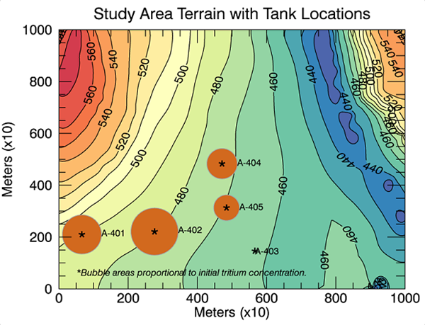
Create some basic visual output to characterize the study area - start by building the base terrain contour plot. We will also use SCATTERPLOT and BUBBLEPLOT to overplot the well locations and initial tritium concentrations once the contouring is complete.
myCT = COLORTABLE(74, /REVERSE)
index = [420,430,440,450,460,470,480,490,500,510, $
520,530,540,550,560,570,580]
myContour = CONTOUR(grid, RGB_TABLE=myCT, $
C_VALUE=index, ASPECT_RATIO=.75, /FILL, $
TITLE="Study Area Terrain with Tank Locations", $
XTITLE="Meters (x10)", YTITLE="Meters (x10)")
myContour2 = Contour(grid, COLOR='black', $
C_VALUE=index, ASPECT_RATIO=.75, /OVERPLOT)
myContour.TITLE.FONT_SIZE = 14
xLoc = [66,276,566,471,484]
yLoc = [210,221,146,483,313]
zLoc = [490,483,470,480,475]
i_tritium = [7, 9, 0, 5, 4]
labels = ['A-401','A-402','A-403','A-404','A-405']
tritium = BUBBLEPLOT(xLoc, yLoc, MAGNITUDE=i_tritium,
EXPONENT=0.75, /OVERPLOT, LABELS=labels,
LABEL_FONT_SIZE=8, LABEL_ALIGNMENT=0.0, $
COLOR='chocolate', LABEL_POSITION='right')
myPlot = SCATTERPLOT(xLoc, yLoc, /OVERPLOT, SYMBOL='*', $
SYM_SIZE=1, SYM_FILLED=1, SYM_THICK=2, SYM_FILL_COLOR='black')
areaText = TEXT(50, 50, TARGET=myPlot, $
'*Bubble areas proportional to initial tritium concentration.', $
/DATA, COLOR='black', FONT_SIZE=8, FONT_STYLE='italic')
At this point in the process your output should look something like the following, assuming you chose to use the parameters in the examples. The initial plot displays the filled terrain contours with well locations plotted and labeled, and a visual representation of the magnitude of the initial concentrations of tritium found in each well at time T0.
Other Topics in this Series
See Also
ASCII_TEMPLATE, COLORTABLE, CONTOUR, Formatting IDL Graphics Symbols and Lines, GRIDDATA, READ_ASCII, READ_CSV, SCATTERPLOT, TEXT