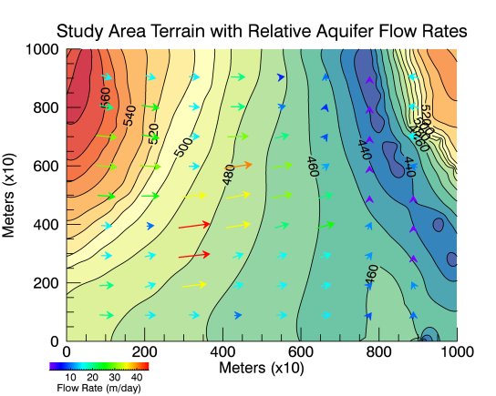
An additional characteristic of the site we could characterize is the relative flow rates of the of the aquifer across the study area. This example uses GRIDDATA and CONTOUR to generate the base terrain map, over which we lay a VECTOR plot of the aquifer flow rates. Your final plot should look similar to this:
Grid the Terrain Data
Using the data in the files "TankTerrainData.csv" (see Model the Study Area and Setting), create a contour plot of the terrain to act as a base for the flow vectors.
Start by reading in the base data to use throughout the rest of the examples. The data resides in the file TankDataTerrain.csv in the \examples\data directory of your IDL installation. This file contains the surface terrain data of our site, in X, Y, Z coordinates (all in meters). The fourth column of data in this file contains the elevation of the surface of the underlying aquifer.
In this example, we create a template with ASCII_TEMPLATE, then read in the data using READ_ASCII.
myTemplate = ASCII_TEMPLATE()
site = READ_ASCII('TankDataTerrain.csv', $
TEMPLATE=myTemplate)
grid = GRIDDATA(site.X, site.Y, site.Z, $
DIMENSION=1000, METHOD="Kriging")
Create the Base Contour Map
Create the plot that will serve as a base for the flow vectors.
myCT = COLORTABLE(74, /REVERSE)
index = [420,430,440,450,460,470,480,490,500,510, $
520,530,540,550,560,570,580]
myContour = CONTOUR(grid, RGB_TABLE=myCT, $
C_VALUE=index, ASPECT_RATIO=.75, /FILL, $
TITLE="Study Area Terrain with Tank Locations", $
XTITLE="Meters (x10)", YTITLE="Meters (x10)")
myContour2 = CONTOUR(grid, COLOR='black', $
C_VALUE=index, ASPECT_RATIO=.75, /OVERPLOT)
myContour.TITLE.FONT_SIZE = 14
Read and Grid the Flow Data
Now that we have the base CONTOUR plot completed, read in the aquifer flow data and create a VECTOR plot in the current window.
Note: The rate of flow for the river is several orders of magnitude greater than that in the aquifer. For this reason, only directional data for river flow is included in the dataset.
myTemplateAQ = ASCII_TEMPLATE()
gwFlow = READ_ASCII('GWFlowRates.csv', TEMPLATE=myTemplateAQ)
myVectors = VECTOR(gwFlow.U, gwFlow.V, gwFlow.AX, gwFlow.AY, $
XRANGE=[0,9], YRANGE=[0,10], rgb_table = 34, /CURRENT, $
AUTO_COLOR=1, background_transparency=100)
ax = myVectors.AXES
ax[0].HIDE= 1
ax[1].HIDE= 1
cb = COLORBAR(TARGET=myVectors, POSITION=[0.10,0.065,0.3,0.085], $
TITLE='Flow Rate (m/day)', FONT_SIZE=8)
Other Topics in this Series
See Also
ASCII_TEMPLATE, COLORBAR, COLORTABLE, CONTOUR, Formatting IDL Graphics Symbols and Lines, GRIDDATA, READ_ASCII, READ_CSV, VECTOR